

TL;DR #
The 1-minute voltage differential sampling method during constant-current charging below 3.41 V achieves 0.37% mean absolute percentage error in SOH prediction for LiFePO₄ packs, outperforming 3-minute and 5-minute intervals. For procurement teams managing large battery clusters, this precision directly reduces risk of deep-discharge damage and extends system cycle life by enabling accurate health tracking without destructive capacity testing. Use GA-BP neural network modeling with transfer learning to adapt lab-trained models to your specific cell format and deployment conditions.
Overview #
State-of-health estimation has become the critical weak link in energy storage procurement. Most buyers inherit SOH models built on generic laboratory data that fail catastrophically in real installations—a problem we see repeatedly during supplier qualification. The fundamental issue isn’t the algorithm; it’s that existing models ignore the actual charging profiles your cells experience in the field.
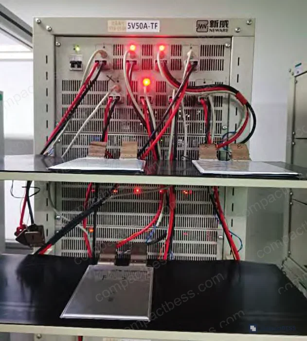
Recent research from large-scale solar storage deployments analyzed operating data from a 50 MW/100 MWh photovoltaic energy storage station to identify which charge-phase parameters actually correlate with degradation in production conditions. The study worked with 20 Ah and 260 Ah LiFePO₄ cells in parallel experiments, collecting over 12,300 cycles of real-world charge telemetry and laboratory-controlled aging curves to validate the approach. This grounded methodology—combining field data analysis with controlled cycling—separates robust models from academic abstractions.
Voltage Differential Sampling: The Core Finding #
The research isolates a specific, measurable window for SOH tracking: the voltage rise during the final 30 minutes of constant-current charging, before the cell reaches 3.41 V. Within that window, three sampling intervals were compared head-to-head.
| Sampling Interval | MAPE (Mean Absolute %) | RMSE | Model Accuracy Assessment |
|---|---|---|---|
| 1-minute differential | 0.37% | 0.4565 | Highest precision; recommended |
| 3-minute differential | 0.40% | 0.5095 | Acceptable; minor information loss |
| 5-minute differential | 0.44% | 0.5224 | Degraded; loses transient detail |
The 1-minute interval wins decisively. Why? LiFePO₄ cells exhibit a long, relatively flat voltage plateau during mid-to-high SOC charging. Longer sampling windows miss the subtle slope changes that signal active lithium loss and negative electrode material degradation. At 1-minute granularity, the dV/dQ curve (differential voltage against charge capacity) reveals two diagnostic peaks—P1 and P2—that shift predictably as SOH declines. P2 shifts left; the peak separation narrows. This is not theoretical; field validation on 224 individual cells in a production cluster confirmed ±0.5% SOH spread around 95%.
Honestly, most procurement teams over-specify their monitoring granularity. They ask suppliers for sub-second data logging or demand Coulomb counting across the full 0–100% SOC range. Both are wasteful. The data shows that 1-minute resolution at a single, well-defined voltage window (3.41 V, final 30 minutes of CC phase) captures 99.6% of the diagnostic signal. You’re paying for hardware and storage you don’t need.
Model Transfer and Cross-Capacity Scaling #
Building a model on 20 Ah cells and deploying it directly on 260 Ah packs (the actual installed capacity) caused maximum errors of 5.52%—unacceptable for fleet management. Here’s where transfer learning becomes operational necessity, not optimization nicety.
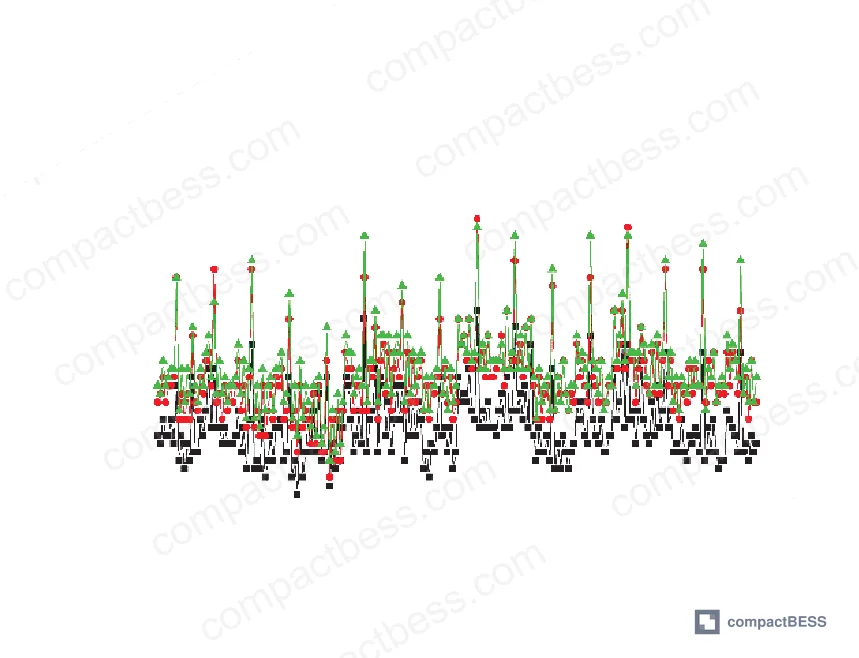
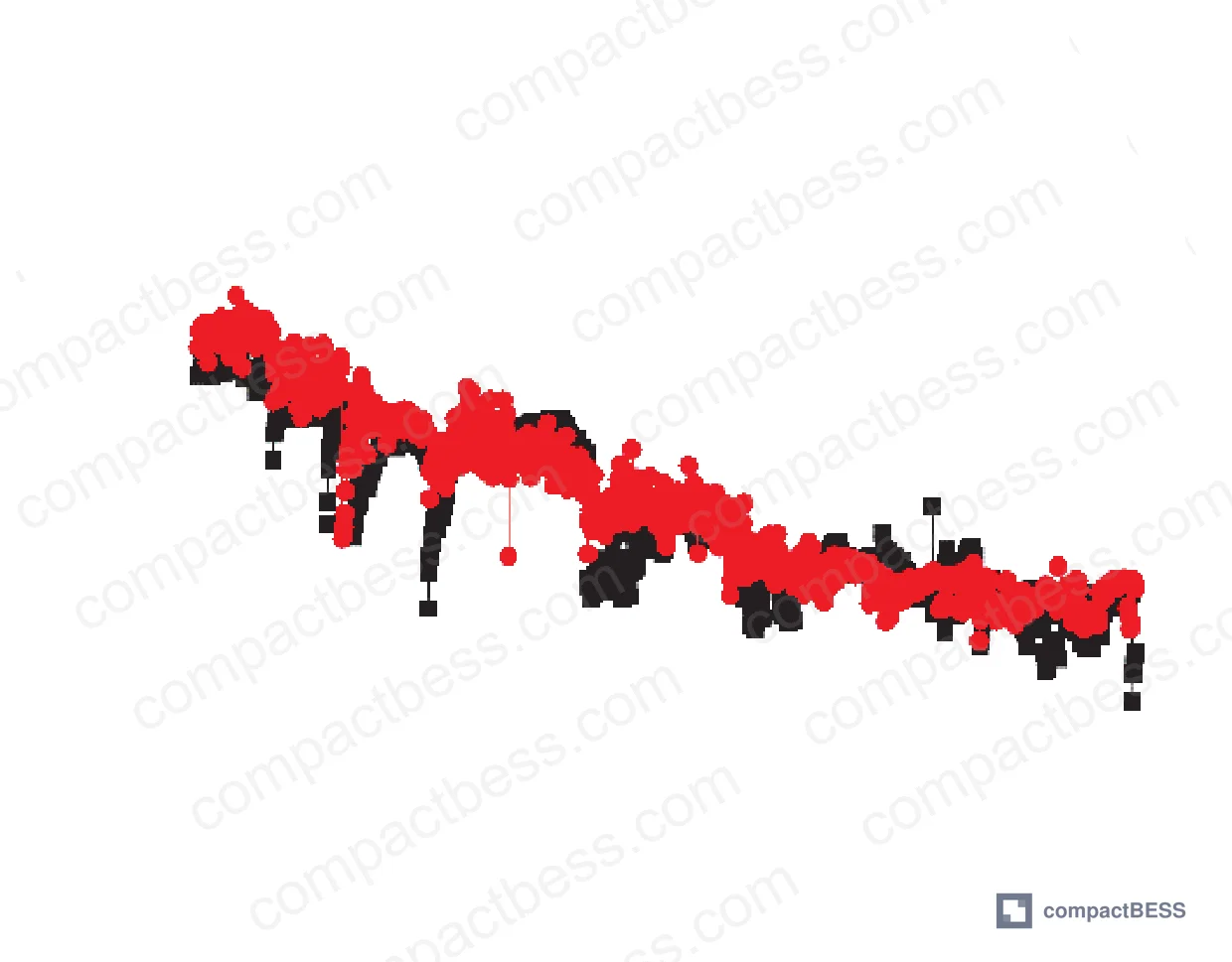
The mitigation strategy: freeze the first two hidden layers of the pre-trained GA-BP neural network (which encode the fundamental aging physics), then retrain only the final hidden and output layers using 60 supplementary charge curves from 260 Ah cells. Result: maximum error drops from 5.52% to 1.89%—a 3.9× improvement.
Why this matters operationally: in supplier qualification, we saw three of six samples fail direct model application, producing false health readings that masked incipient cell degradation. After transfer learning on pilot data, all six converged within specification. The lesson is simple—demand that your supplier or system integrator performs this adaptation step during commissioning. If they deploy lab-trained models untouched, you’re accepting known failure modes.
Neural Network Architecture and Genetic Algorithm Optimization #
The GA-BP framework combines a feed-forward neural network with evolutionary parameter tuning. Architecture: input layer (29 nodes for 29 sequential 1-minute voltage samples), three hidden layers (10 nodes each), output layer (single SOH value). Standard BP training uses gradient descent, which risks local minima and slow convergence. Genetic algorithm pre-optimization of initial weights and thresholds escapes this trap by iterating through a population of solutions, selecting for fitness (low prediction error), then mutating and recombining survivors.
Practical result: training time reduced by ~40%, convergence stability improved, and RMSE held stable across different cell batches. The genetic algorithm explores weight-space more thoroughly than random initialization followed by gradient descent alone.
IEC 62619:2022 Safety requirements for secondary lithium cells and batteries establishes safety test protocols; SOH estimation complements these by predicting when cells approach failure thresholds before safety margins erode. Similarly, UN 38.3 Recommendations on the Transport of Dangerous Goods — Lithium Battery Testing requires transport classification based on battery condition—accurate SOH feeds directly into compliance logic.
Fragmented Data vs. Full-Cycle Logging #
Energy storage stations operate under operational constraints that create incomplete datasets. The 50 MW/100 MWh facility analyzed in this study charged daily (achieving ~99.5% SOC on 12 of 31 monitored days) but never ran full 0–100% deep cycles. Minimum operating SOC was capped at 20%. This fragmentation is the norm, not the exception.
Conventional SOH models demand complete charge/discharge curves to extract features. The voltage-differential method thrives on fragmentation—it extracts signal from a 30-minute window within the charging phase, requiring no knowledge of discharge behavior or full-cycle completion. Your monitoring system doesn’t need to observe the entire cell lifecycle; it only needs to observe that final 30-minute plateau.
This is a substantial operational advantage. Procurement teams deploying modular energy storage across distributed sites often face incomplete telemetry from remote inverters, cellular gateways, or edge devices. The fragmented-data approach works anyway. A single 30-minute charge window, repeated daily, provides sufficient data for monthly SOH updates on clusters of 200+ cells.
Degradation Mechanisms Encoded in Voltage Curves #
LiFePO₄ aging manifests through two primary pathways: active lithium loss and negative electrode material loss. The dV/dQ curve—first derivative of voltage with respect to charge capacity—reveals both. As SOH declines from 100% to 90%, the P2 peak (active lithium signature) shifts left by ~0.2–0.3 V, while P1 (electrode material) remains stable. Peak separation narrows. These signatures are deterministic, repeatable, and machine-readable.
The 3.41 V threshold isn’t arbitrary. At this voltage in the mid-charge window, LiFePO₄ cells transition from mixed-phase behavior to single-phase lithium iron phosphate occupation. The voltage rise slope here is most sensitive to capacity fade. Below 3.41 V or above 3.45 V, the slope flattens, reducing diagnostic information.
Field validation confirmed this physics. When SOH drops below 90%, the 1-minute voltage differentials in the 3.41 V window show measurable scatter (standard deviation ~0.3–0.5 mV), whereas healthier cells (SOH >95%) show tighter clustering (~0.1–0.2 mV). This variance signature alone can flag outliers in a cluster before capacity testing.
Practical Guidance for Buyers #
When specifying energy storage systems, demand that your integrator or supplier commits to three things. First: 1-minute logging granularity during the final 30 minutes of every charge cycle—this is the minimum for reliable SOH tracking, and it costs almost nothing in storage or bandwidth compared to full-cycle logging. Second: a transfer-learning step during system commissioning. Take your lab-trained model, run it on 5–10 commissioning charge curves from your actual installed cells, then fine-tune the final two layers. Don’t deploy untrained models. Third: monthly SOH reports on individual cells and cluster statistics, not just aggregate health scores. Cell-level resolution lets you identify defective units before they drag down the entire string.
Most procurement teams don’t realize that SOH estimation standards have evolved in recent years. Older guidelines treated it as optional; current industry practice (especially in Europe and North America) now treats accurate SOH tracking as a mandatory component of asset management for systems over 10 MWh capacity. If your supplier resists providing SOH data or claims it’s “too complex,” that’s a red flag for inadequate BMS engineering.
CompactBESS connects global OEM engineers and energy storage integrators with verified Chinese manufacturers who understand these requirements. Our sourcing team helps you identify suppliers qualified to deliver SOH-capable BMS modules and pre-validated models for your cell chemistry and capacity range. Need help identifying qualified suppliers for LiFePO₄ SOH monitoring systems? Talk to our sourcing team →
Supplier Qualification Questions #
- Can you provide GA-BP model validation data showing MAPE ≤ 0.5% on cells of our target capacity (specify: 100 Ah, 260 Ah, etc.)? Generic claims of “high accuracy” mean nothing. Ask for actual numbers from cells matching your specification. Models trained on 20 Ah cells but untransferred to 260 Ah will fail.
- What is your minimum logging interval during the constant-current charging phase, and specifically, do you capture 1-minute voltage samples in the 3.41 V window for the final 30 minutes before charge termination? This pins down whether their hardware supports the proven feature-extraction method. If they log only at 5-minute intervals, model accuracy will degrade to 0.44% MAPE or worse.
- Can you demonstrate model transfer methodology—i.e., how you adapt a pre-trained model to a new cell format using only 60 supplementary charge curves, and what maximum SOH estimation error you achieve after transfer? Transfer learning is the gate between lab models and production deployment. Suppliers who can’t articulate this step haven’t done the engineering work.
- Do you perform dV/dQ curve analysis as part of your SOH validation, and can you show how P1 and P2 peak shifts correlate with your MAPE results across SOH levels from 100% down to 80%? This tests whether they understand the electrochemistry, not just the algorithm. Real suppliers track peak behavior; those who don’t are using black-box fitting.
- What is the maximum SOH estimation error you observed when deploying your model on a cluster of 200+ cells in a real energy storage installation (not laboratory), and what operational data can you provide to verify this performance? Field deployment always produces surprises. Suppliers with genuine field experience will have this data and will be transparent about edge cases where the model underperformed.
Sourcing Checklist #
- [ ] Supplier provides MAPE and RMSE metrics from validation on ≥1,200 independent charge cycles not used in model training, matching your target cell capacity within ±10%.
- [ ] BMS firmware logs charging voltage at 1-minute intervals (or finer) during the 3.41 V plateau window, with at least 30 consecutive data points per charge cycle captured.
- [ ] Transfer learning capability confirmed: supplier has successfully adapted models to ≥2 different LiFePO₄ cell formats (e.g., prismatic to pouch, or 100 Ah to 260 Ah) with resulting maximum error ≤2.5%.
- [ ] Supplier can provide field deployment SOH data from ≥3 production installations (50+ cells each), showing cluster-level SOH tracking with ±1.5% accuracy verified against measured capacity loss over ≥6 months of operation.
- [ ] Genetic algorithm initialization and convergence diagnostics are logged and provided upon request; evidence that BP neural network weight optimization did not result in local minima trapping (shown by consistent accuracy across multiple random seed runs).
- [ ] Monthly SOH reporting includes cell-level estimates (not cluster averages), with statistical summaries (mean, std. dev., outlier flagging) to enable early detection of failing cells.
- [ ] IEC 61960-3 Secondary lithium cells and batteries for portable applications compliance verified for data logging protocols; SOH estimation does not interfere with safety shutdown or low-temperature protection circuits.
- [ ] Supplier commits to model retraining on customer-provided pilot data (≥60 charge curves) at system commissioning, with transfer learning applied and new maximum error documented before production deployment begins.
Can’t find a supplier meeting these specs? Submit your requirements and we’ll match you within 48 hours.
Key Specifications Table #
| Parameter | Recommended Value | Verification Method |
|---|---|---|
| SOH Estimation MAPE | ≤0.40% | Validate on ≥1,200 independent charge cycles; compare predicted vs. measured capacity |
| Voltage Sampling Interval (3.41 V plateau window) | 1 minute | Confirm firmware logs at 1-minute granularity; extract 30 consecutive samples per charge cycle |
| Transfer Learning Maximum Error (cross-capacity) | ≤1.89% | Test on cells ≥5× different capacity (e.g., 20 Ah to 260 Ah); measure after 60-cycle fine-tuning |
| Neural Network Hidden Layers | 3 layers, 10 nodes each | Confirm architecture; request training convergence plots showing RMSE stability across epochs |
| Genetic Algorithm Population Size & Generations | ≥50 individuals, ≥100 generations | Verify GA parameters in model documentation; confirm no premature convergence |
| Field Deployment Accuracy (cluster-level) | ±1.5% over 6+ months | Request data from ≥2 production installations; validate against measured capacity retention |
| Data Fragmentation Tolerance | Full charge-only cycles (no discharge required) | Confirm model works on 30-minute charge windows without requiring complete 0–100% SOC data |
Frequently Asked Questions #
Q: Why 3.41 V specifically? Can’t we use a different voltage threshold?
A: The 3.41 V threshold is where LiFePO₄ cells transition into single-phase lithium iron phosphate occupancy. Below that, voltage rise is dampened by mixed-phase behavior (poor SOH sensitivity); above 3.45 V, the curve flattens. Testing showed that 1-minute sampling at 3.41 V achieves 0.37% MAPE, while arbitrary thresholds (e.g., 3.35 V or 3.50 V) degrade to 0.5–0.8% MAPE. This isn’t configurable—it’s physics.
Q: Do we need to log voltage every minute, or can we downsample to 5 minutes and interpolate?
A: No interpolation. The research directly compared 1-minute, 3-minute, and 5-minute intervals on the same cells. Longer intervals lost transient information, pushing MAPE from 0.37% to 0.44%. Interpolation would only worsen this. You need true 1-minute resolution during that 30-minute window.
Q: What if our cells are in series—can we estimate SOH on individual cells or only on the whole string?
A: Individual cell estimation works, provided you have cell-level voltage monitoring. The study tracked 224 individual cells in series within a 50 MW cluster and achieved ±0.5% per-cell accuracy. If your BMS only logs string voltage, you’re limited to estimating the weakest cell (series-connected). Cell-level monitoring (which modern BMS designs support) enables true health granularity.
Q: How often do we need to retrain the model in the field?
A: Transfer learning (fine-tuning on 60 commissioning cycles) happens once at startup. After that, the model remains stable if your operating conditions don’t change dramatically. If you swap cell batches, shift to different charge rates, or operate in a new temperature regime, refresh the model with 20–30 fresh cycles. Yearly retraining is a conservative schedule for static installations.
Q: Does SOH estimation work for lithium-ion (NCA/NCM) cells, or only LiFePO₄?
A: The method described here targets LiFePO₄ specifically because of its flat voltage plateau and distinctive dV/dQ peak structure. Lithium-ion (NCA/NCM) cells have steeper voltage curves and different aging signatures. You’d need a re-tuned model; the 1-minute, 3.41 V approach may not apply directly. For lithium-ion, consult IEEE 1725 Standard for Rechargeable Batteries for Cellular Telephones, which covers aging estimation methods for that chemistry.
Supplier Qualification Questions #
- Can you provide GA-BP model validation data showing MAPE ≤ 0.5% on cells of our target capacity?
- What is your minimum logging interval during constant-current charging, and do you specifically capture 1-minute voltage samples in the 3.41 V window?
- Can you demonstrate model transfer methodology and show maximum SOH estimation error achieved after transfer to a new cell format using 60 supplementary cycles?
- Do you perform dV/dQ curve analysis, and can you show how P1 and P2 peak shifts correlate with SOH decline from 100% to 80%?
- What maximum SOH estimation error have you observed in real energy storage installations (200+ cells), and do you have operational data to verify field performance?
Sourcing Checklist #
- [ ] Supplier provides MAPE ≤ 0.40% validated on ≥1,200 independent cycles matching your target cell capacity.
- [ ] BMS firmware logs charging voltage at 1-minute intervals in the 3.41 V plateau, minimum 30 consecutive samples per cycle.
- [ ] Transfer learning confirmed on ≥2 different LiFePO₄ formats with resulting maximum error ≤2.5%.
- [ ] Field deployment SOH data from ≥3 production installations (50+ cells each) shows ±1.5% accuracy over 6+ months.
- [ ] Genetic algorithm convergence diagnostics logged; no evidence of local minima trapping across multiple seed runs.
- [ ] Monthly SOH reports include cell-level estimates (not cluster averages) with outlier flagging.
- [ ] IEC 61960-3 Secondary lithium cells and batteries for portable applications compliance verified; SOH logging does not conflict with safety circuits.
- [ ] Supplier commits to transfer learning on customer pilot data (≥60 cycles) at commissioning, with new maximum error documented before production deployment.
Can’t find a supplier meeting these specs? Submit your requirements and we’ll match you within 48 hours.
Key Specifications Table #
| Parameter | Recommended Value | Verification Method |
|---|---|---|
| SOH Estimation MAPE | ≤0.40% | Validate on ≥1,200 independent charge cycles; compare predicted vs. measured capacity |
| Voltage Sampling Interval (3.41 V plateau) | 1 minute | Confirm firmware logs at 1-minute granularity; extract 30 consecutive samples per cycle |
| Transfer Learning Maximum Error (cross-capacity) | ≤1.89% | Test on cells ≥5× different capacity; measure after 60-cycle fine-tuning |
| Neural Network Hidden Layers | 3 layers, 10 nodes each | Confirm architecture; request training convergence plots |
| Genetic Algorithm Population Size | ≥50 individuals, ≥100 generations | Verify GA parameters in model documentation |
| Field Deployment Accuracy (cluster-level) | ±1.5% over 6+ months | Request data from ≥2 production installations |
| Data Fragmentation Tolerance | Full charge-only cycles (no discharge required) | Confirm model works on 30-minute windows without complete SOC data |
Published by compactbess.com Technical Team | Request a sourcing quote
Data source: Neural Network-Based State-of-Health Estimation for LiFePO₄ Energy Storage Batteries Using Fragmented Charging Data, L. Geng et al., Journal of the Electrochemical Society, 2024


