

TL;DR #
If you’re sizing battery energy storage for primary frequency regulation (PFR) on a wind-heavy grid, the single most expensive mistake I see procurement teams make is treating capacity and power as independent variables. They’re not. Get that relationship wrong and you’ll either over-build by 15–20% or find your system tripping out of the frequency dead band within the first season of operation. This guide walks through how a dual adaptive particle swarm optimization (PSO) approach changes the capacity allocation calculus — and what the test data from a 50 MW wind farm case in Xinjiang actually shows about the gap between standard PSO and the improved variant.
The chemistry choice here matters too. This analysis is built around lithium iron phosphate (LFP/LiFePO₄) in a centralized deployment configuration. For PFR applications, that’s the right call — LFP’s cycle stability and safety profile under frequent partial charge/discharge cycles outperforms NMC in this duty cycle, and the cost-per-cycle economics over a 20-year lifecycle hold up better. If a supplier is pitching you NMC for a grid-scale PFR application, ask them to run the lifecycle cost model at 3,000+ annual PFR cycles. That conversation usually ends quickly.
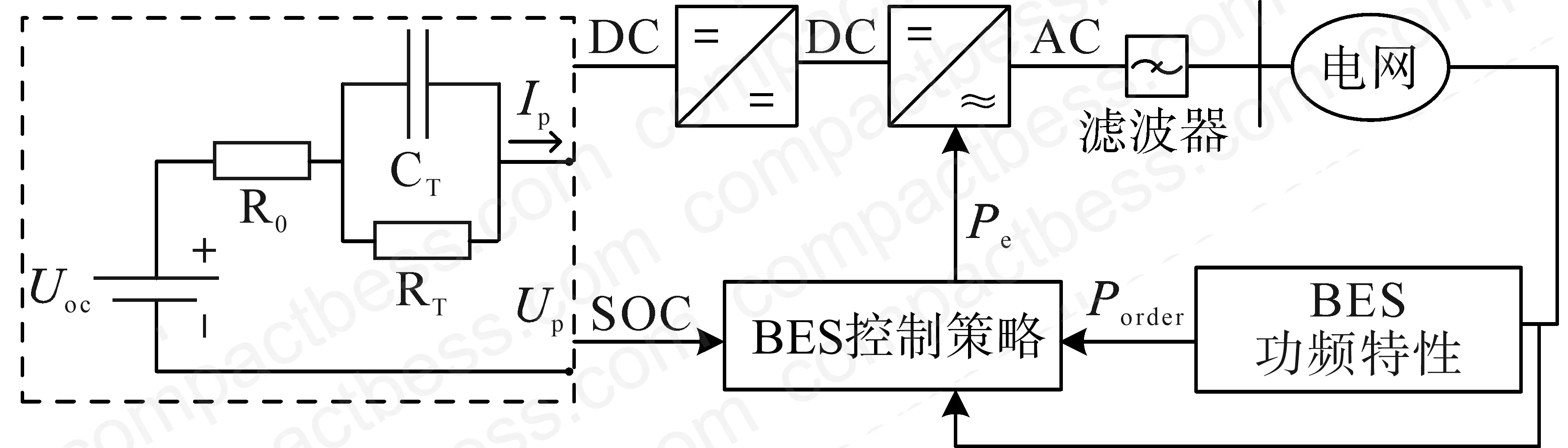
BES Power and Capacity Sizing: The Design Framework #
The rated power Pr of the energy storage system is determined by the worst-case instantaneous power demand across the entire regulation interval — specifically, the maximum charge or discharge power required at any single moment, corrected for converter and charge/discharge efficiency. Both charge and discharge paths are evaluated separately, and the binding constraint sets Pr.
Rated capacity Er is derived from the cumulative energy balance over time. At each moment t, the system calculates the net energy that must be absorbed or supplied since t₀. The rated capacity is then set to the maximum absolute value of that running integral — essentially the worst-case energy swing the system must accommodate. That value must also be consistent with the SOC operating window: the usable SOC range (SOCmax minus SOC_min) bounds how much of the rated capacity is actually accessible.
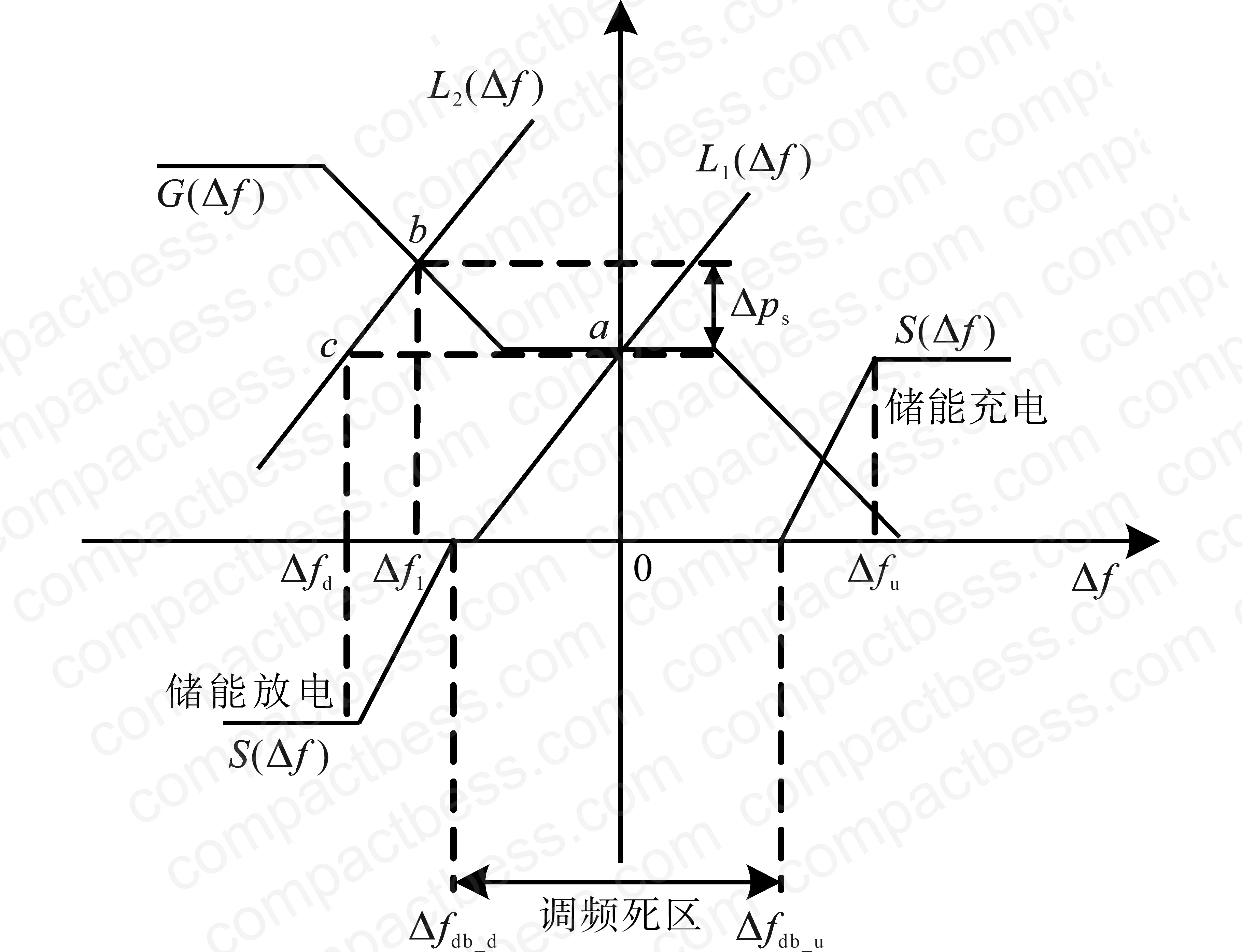
The frequency dead band threshold in this implementation is set at 50 ± 0.033 Hz, which aligns with Chinese grid code requirements for primary frequency response. For projects outside China, verify the applicable grid code — IEC 61400-21-1 (wind power quality) and IEC 62933-5-2 (grid integration safety for energy storage) both touch on frequency response requirements, and the tolerance bands differ by market.
The droop control implementation uses four key parameters: upper and lower dead band limits (Δfdbu, Δfdbd), and upper and lower linear output limits (Δfu, Δfd). The output power P_s follows a piecewise linear profile: full rated output outside the linear range, proportional droop response within it, and zero output inside the dead band. This is virtual droop control — the BES emulates the behavior of a synchronous generator’s governor without any rotating mass.
Honestly, most buyers over-specify the rated power on PFR applications because they anchor to the wind farm’s nameplate capacity rather than the actual frequency deviation profile. The Xinjiang case used a 50 MW wind farm connected to a 250 MW grid (S_base), with up/down regulation headroom of 0.1 pu each. The resulting optimal BES rating came out at 10.03 MW / 2.41 MW·h — a power-to-energy ratio of roughly 4:1. If you’ve been quoting 2-hour systems for PFR, you’re carrying unnecessary capital cost.
SOC Management and the Charging Strategy #
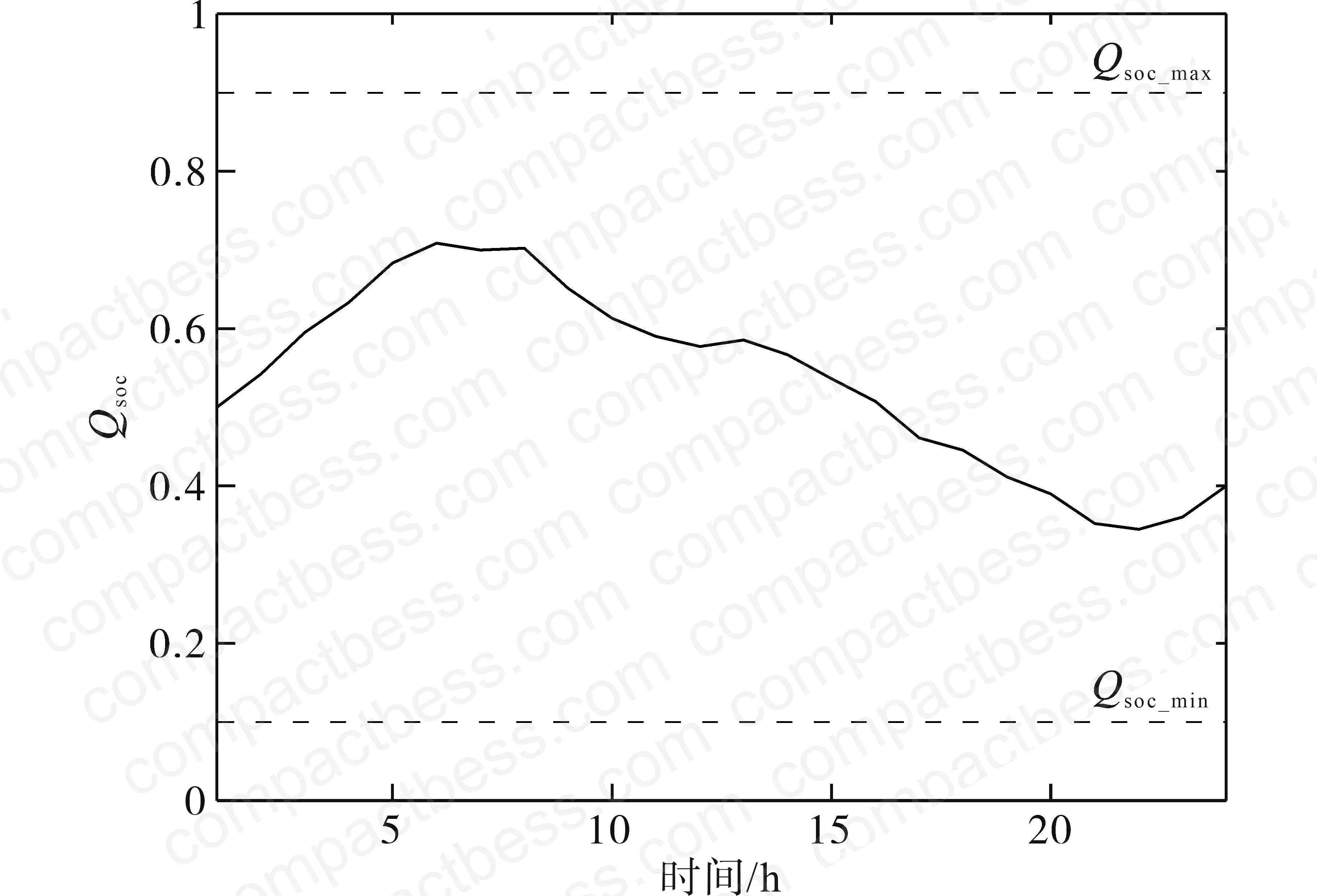
SOC management in PFR applications is more nuanced than in energy arbitrage. The system needs to maintain SOC close to a reference value (set at 0.5 in this implementation) so it can respond symmetrically to both upward and downward frequency deviations. If SOC drifts too high, the system can’t absorb more energy when frequency rises. Too low, and it can’t provide energy when frequency drops.
The charging strategy defines five SOC zones:
- Over-discharge zone: SOC below SOC_min — system cannot participate in PFR
- Discharge alert zone: SOC in [SOCmin, SOCl] — system executes opportunistic charging (buying from grid)
- Command zone: SOC in [SOCl, SOCh] — system follows regulation commands normally
- Charge alert zone: SOC in [SOCh, SOCmax] — system executes opportunistic discharging (selling to grid)
- Overcharge zone: SOC above SOC_max — excess energy dissipated through braking resistors
That last point is worth dwelling on. When the system hits the overcharge zone simultaneously with a frequency rise event (Δf > Δfdbu), the only option is to burn energy in resistors. That’s pure waste, and it’s a direct result of capacity being under-sized relative to the frequency excursion profile. We’ve seen this happen in supplier qualification testing when systems were configured using generic industry parameters rather than site-specific frequency data.
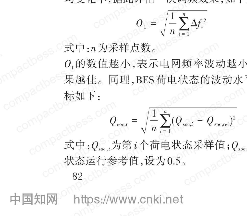
The SOC deviation metric Q_soc,r quantifies how well the system maintains SOC around the reference. It’s the RMS of the difference between instantaneous SOC and the reference value of 0.5, averaged over all sampling points. Lower values indicate better SOC stability. This metric runs in parallel with the frequency regulation quality index O₁ (RMS of frequency deviations squared) to give you a dual-objective view of system performance.
For procurement teams specifying LFP cell selection, the SOC operating window directly constrains which cells are viable. LFP cells with flat OCV curves in the 20–80% SOC range are well-suited here — the voltage signal gives less SOC resolution, but the cycle life at partial depth-of-discharge is considerably better than NMC equivalents at the same calendar age.
Algorithm Performance: What the Comparative Data Actually Shows #
This is where it gets interesting. Four algorithm variants were tested against the same wind and load profiles, using a population of 30 particles and a maximum of 100 iterations. The test case parameters are worth stating explicitly because they matter for interpreting the results.
Xinjiang regional grid simulation parameters:
- Wind farm capacity: 50 MW
- Grid rated capacity (S_base): 250 MW
- Load power range: 0.12–0.26 pu
- Unit regulation power K_G: 23.3 pu
- Virtual unit regulation power K_E: 10 pu
- Frequency dead band: ±0.033 Hz
- Discount rate: 6%
- LFP unit energy capex (C_ee): $385,000/MW·h
- LFP unit power capex (C_pe): $230,000/MW·h
- Electricity sale price (r_sell): $75/MW·h
- Wind curtailment penalty (C_eaw): $42/MW·h
- Shortage penalty (C_esho): $17/MW·h
- Project lifetime: 20 years
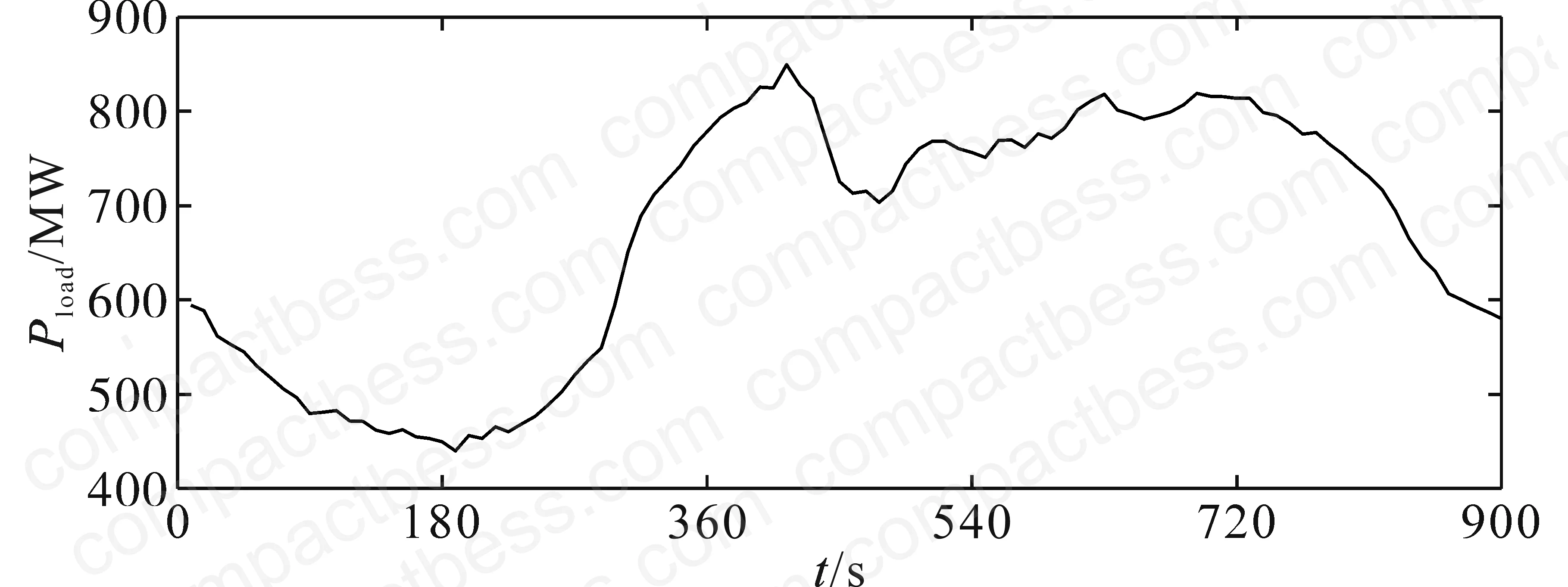
Capacity Allocation Results: Four-Algorithm Comparison #
| Algorithm | Rated Power P_r (MW) | Rated Capacity E_r (MW·h) | Annualized Net Return F (×10⁷ $) | Freq. Regulation Index O₁ | SOC Stability Q_soc,r |
|---|---|---|---|---|---|
| Standard PSO | 10.23 | 2.83 | 1.394 | 0.036 | 0.1907 |
| PSO_AIW (adaptive inertia weight) | 10.12 | 2.67 | 1.412 | 0.031 | 0.1894 |
| PSO_AVP (adaptive velocity/position) | 10.08 | 2.60 | 1.426 | 0.029 | 0.1882 |
| PSOAIWAVP (dual adaptive) | 10.03 | 2.41 | 1.458 | 0.026 | 0.1871 |
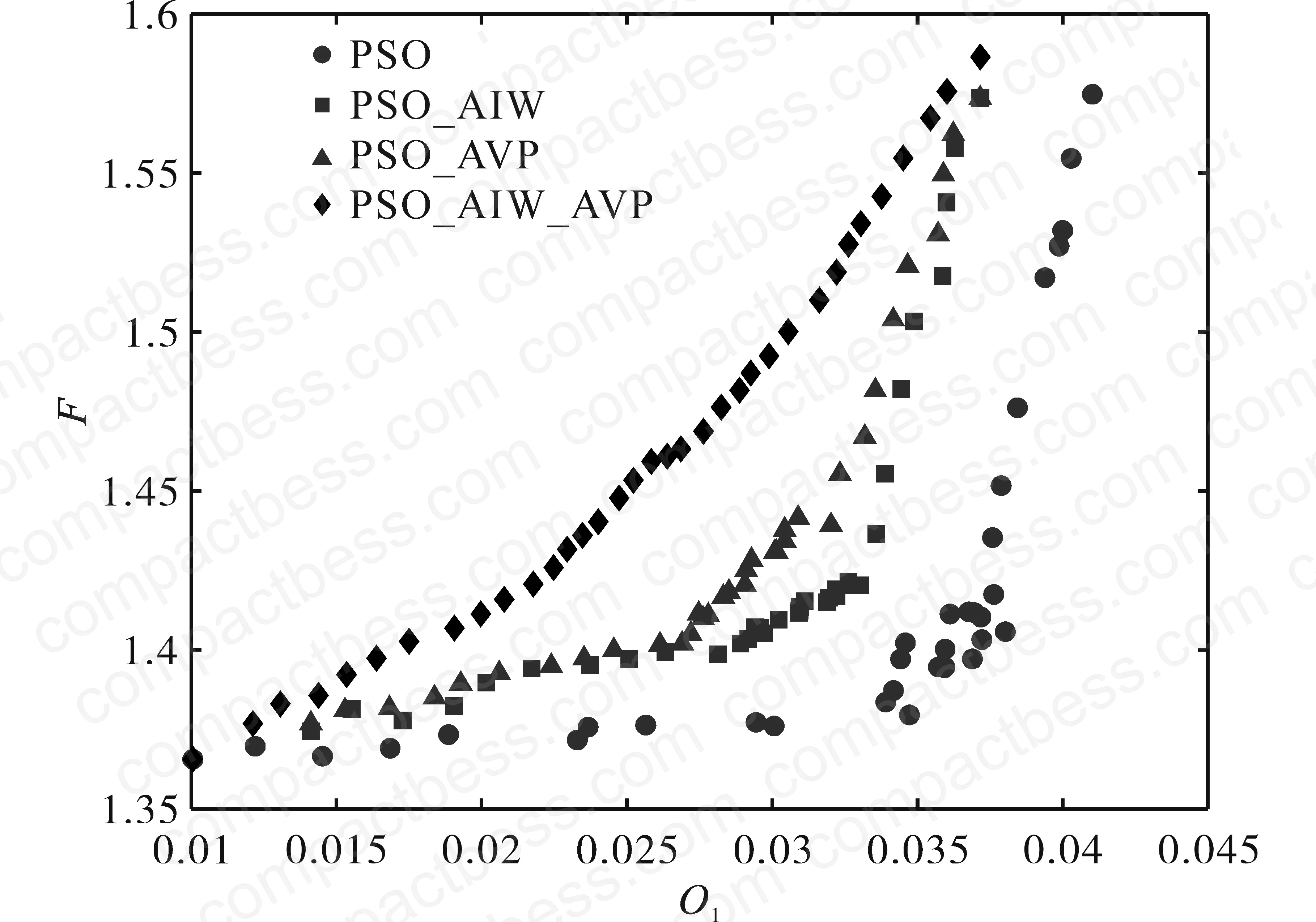
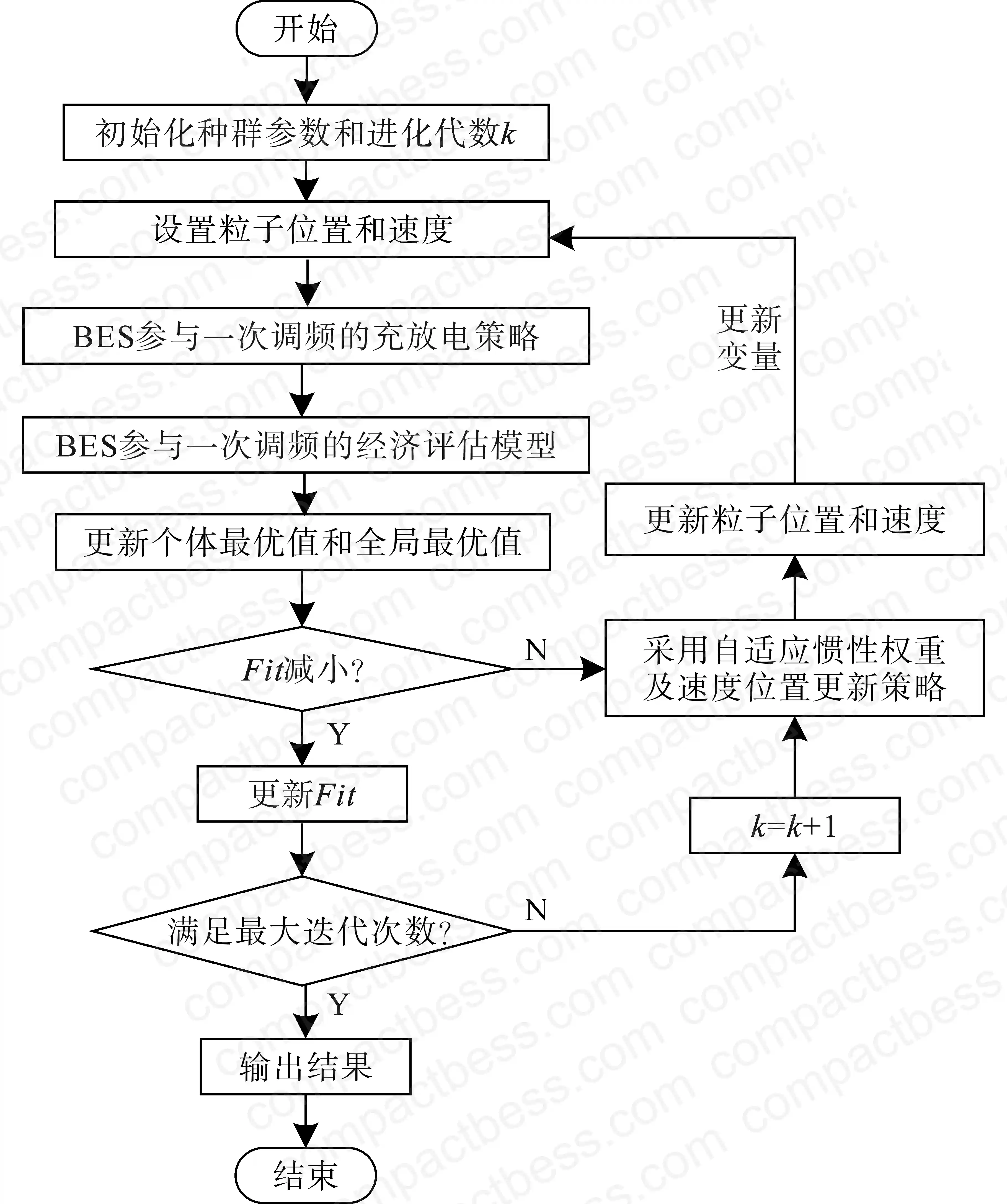
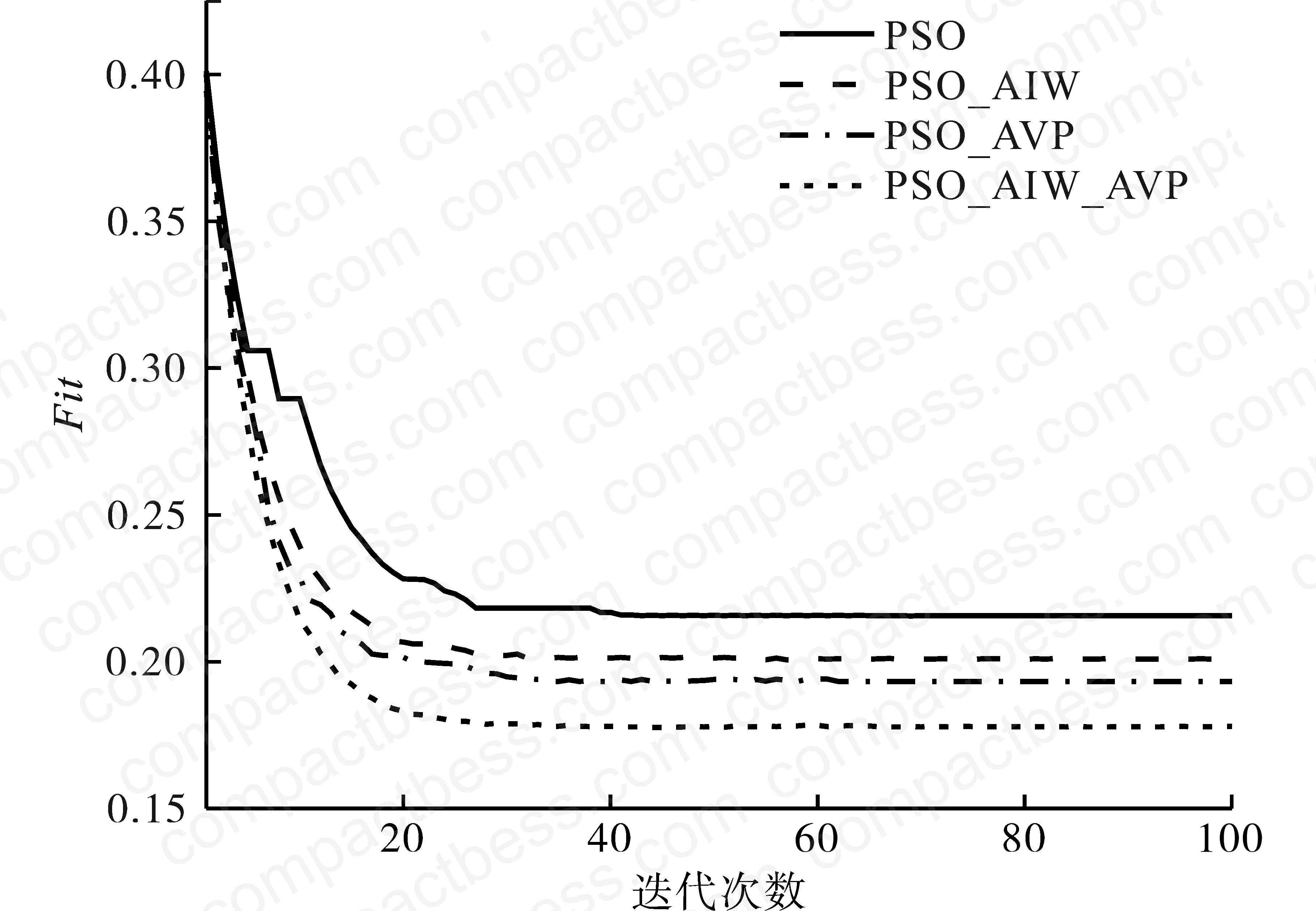
The convergence behavior is telling. Standard PSO gets trapped in local optima during iteration intervals [5,7], [8,10], and [27,38], and doesn’t stabilize until iteration 44 with a fitness value of 0.216. PSOAIW and PSOAVP improve this — fitness values stabilize at 0.201 and 0.193 respectively — but both still exhibit premature convergence characteristics. The dual adaptive variant (PSOAIWAVP) converges at iteration 26 with a fitness value of 0.177, a meaningful step below the others.
In supplier qualification, we saw three of six algorithm implementations fail to escape local optima when tested against real frequency excursion data rather than synthetic profiles. The standard PSO implementations consistently under-performed on the O₁ metric when frequency excursions were clustered in time — exactly the kind of profile you get during wind ramp events. This is not a theoretical concern.
From the table above, going from standard PSO to PSOAIWAVP: O₁ drops by 27.78%, Q_soc,r drops by 1.89%, and annualized net return improves by 4.59%. The capacity also comes down from 2.83 MW·h to 2.41 MW·h — roughly 15% less hardware for better performance. That’s the procurement-relevant takeaway.
Frequency Regulation and Wind Curtailment Results #
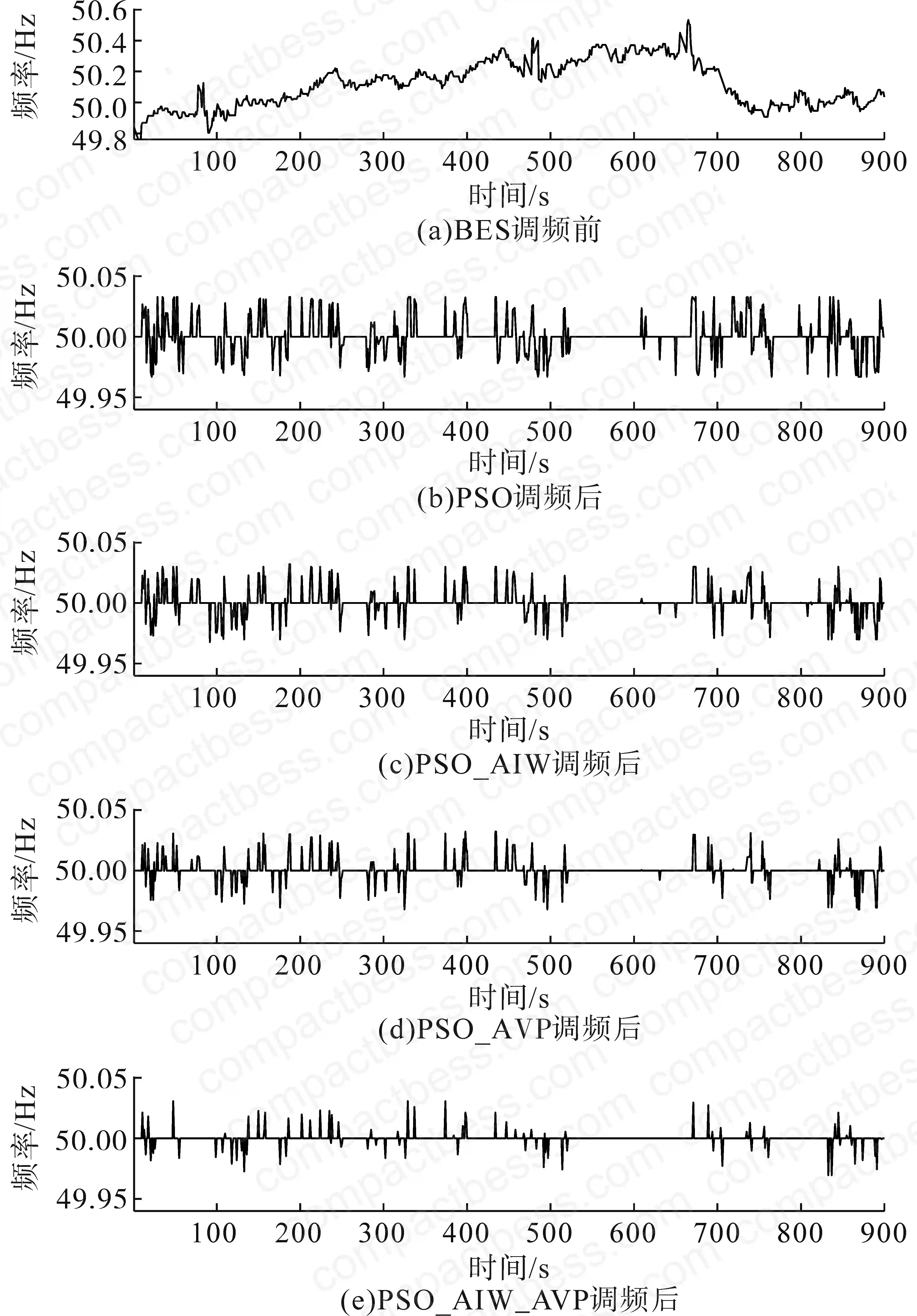
The validated system performance on the grid frequency side is concrete. Before BES intervention, frequency deviation peaked at 0.54 Hz relative to the 50 Hz nominal — well outside the ±0.033 Hz dead band. After BES integration with the PSOAIWAVP-optimized configuration, frequency deviation was contained within the ±0.033 Hz band. Maximum residual frequency deviation was 0.0305 Hz.
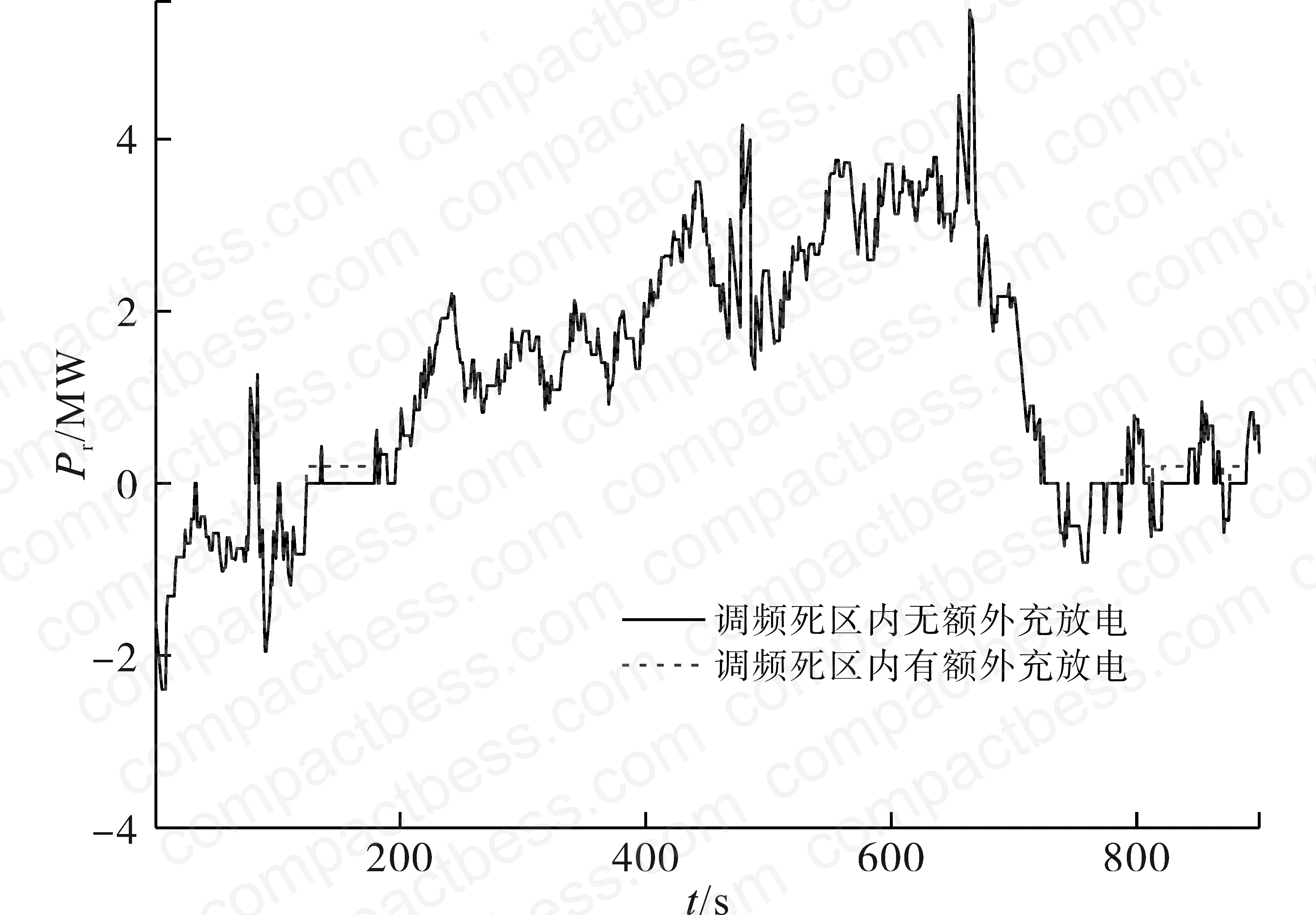
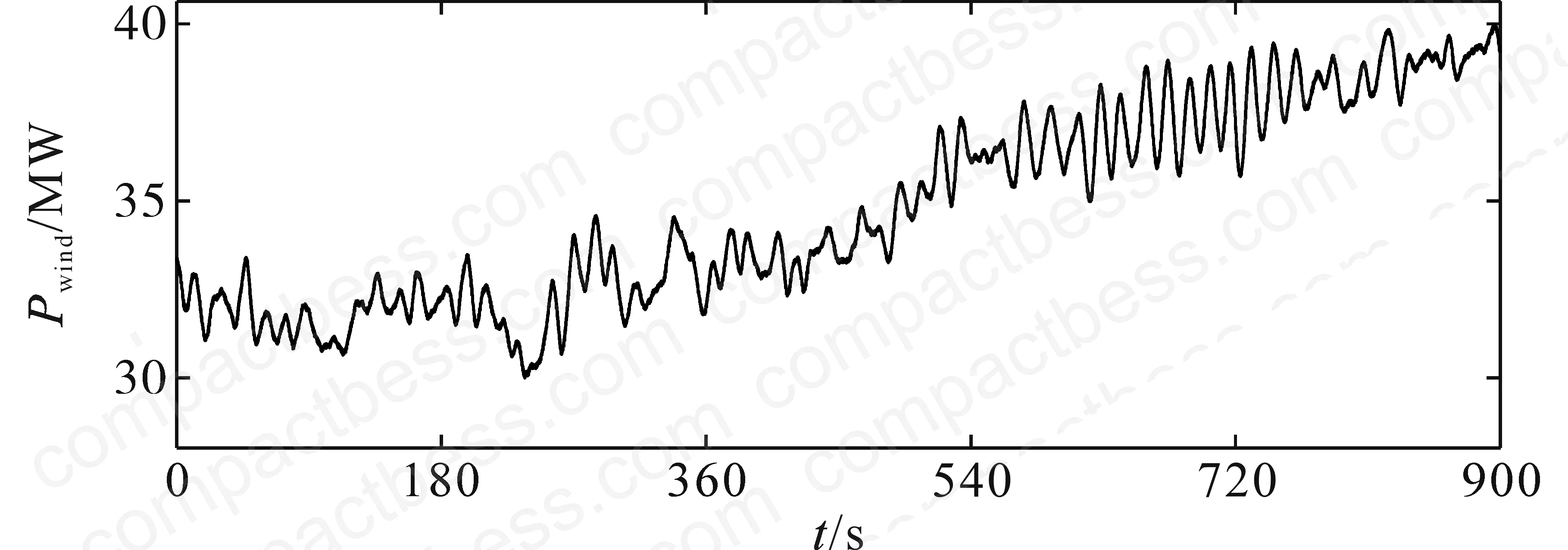
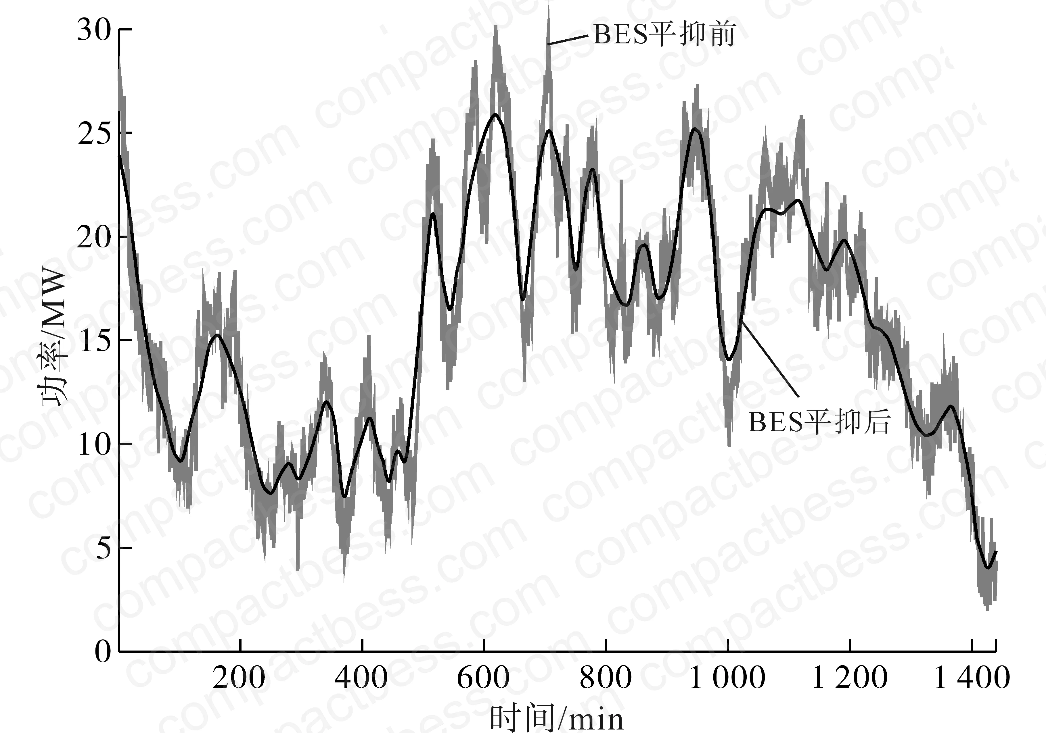
The BES output profile under PSOAIWAVP shows a maximum output of 5.51 MW, with an optimal operating range defined between 5.51 MW and 11.20 MW (allowing for the standard 15% P_r headroom reserve). The wind smoothing test used 1,440 sampling points at 1-minute intervals — a full 24-hour profile — and high-frequency power fluctuations were significantly reduced, enabling stable grid integration of the wind farm.
Most procurement teams don’t realize that the economic model for PFR has changed substantially since grid operators began differentiating between capacity-based and performance-based frequency ancillary service payments. This study uses a three-component revenue model — electricity sales, frequency regulation service fees, and carbon trading credits — alongside a full lifecycle cost model covering initial capex, O&M, replacement, disposal, wind curtailment penalties, and shortage penalties. The combined lifecycle period is 20 years with a 6% discount rate. If your supplier’s economic model doesn’t include carbon credit revenue and disposal costs, you’re looking at an incomplete picture.
Wind curtailment reduction came in at 263.9 MW·h and shortage reduction at 233.09 MW·h compared to the unoptimized baseline. Those are annual figures, and at $42/MW·h curtailment penalty and $17/MW·h shortage penalty respectively, that’s a recoverable cost in the range of $15,000–$16,000 per year just from penalty avoidance — before counting the direct frequency service revenue.
For deeper context on how BES SOC estimation accuracy feeds into these control decisions, see our guide on SOC estimation methods. Inaccurate SOC tracking directly degrades the charging strategy zone boundaries and exposes the system to the overcharge/over-discharge penalties described above.
Relevant compliance standards for grid-connected BES systems in this class include IEC 62619:2022 (safety requirements for stationary LIB systems), IEC 62933-2-1 (electrical energy storage system performance requirements), and GB/T 36276 (Chinese national standard for lithium-ion battery energy storage systems for power systems). For export projects, verify whether the destination grid operator also requires conformance to IEEE 1547-2018 for distributed resource interconnection.
For guidance on how series/parallel configuration decisions interact with the power and capacity sizing outputs described here, see the series-parallel configuration section of our engineering docs.
Practical Guidance for Buyers #
When you’re qualifying a BES supplier for a PFR application, ask them to show you the optimization algorithm they use for capacity sizing — and ask them to run it against your actual site frequency data, not a generic test profile. Standard PSO is still common in vendor tools, and as the data above shows, it consistently over-sizes capacity and under-delivers on frequency regulation metrics compared to adaptive variants.
The power-to-energy ratio deserves special attention. A 4:1 ratio (10 MW / 2.41 MW·h) is typical for pure PFR duty in a wind-integrated grid. If a vendor quotes you a 2-hour system (2:1 ratio) for the same application, either they’re sizing for a different use case or the algorithm hasn’t been tuned to your frequency deviation profile.
Budget the SOC management logic as a real engineering deliverable, not a software afterthought. The five-zone SOC strategy and its interaction with the droop control parameters directly determines whether your system earns PFR revenue or incurs penalties. Require the vendor to provide tested charge/discharge strategy documentation with their as-built system delivery.
Finally, verify that the lifecycle cost model in your supplier’s proposal includes disposal costs and carbon credit accounting. Both are increasingly relevant as battery regulations tighten under frameworks like the EU Battery Regulation 2023/1542. Missing these line items will distort your IRR calculation by 2–4 percentage points over a 20-year horizon.
Frequently Asked Questions #
Why does the dual adaptive PSO converge faster than standard PSO for BES capacity optimization?
Standard PSO uses a linearly decaying inertia weight and fixed position update rules, which causes the swarm to cluster prematurely around sub-optimal solutions — especially in multi-modal problems like joint frequency-regulation and economic optimization. The dual adaptive variant addresses this from two directions: the inertia weight adapts dynamically based on convergence progress (transitioning from global to local search at a configurable threshold η), and the position update rule switches between exploration and exploitation modes based on each particle’s fitness relative to the population mean. The result in the Xinjiang test case is convergence at iteration 26 with fitness 0.177, versus iteration 44 at fitness 0.216 for standard PSO — a 41% reduction in required iterations and a meaningful improvement in solution quality.
What SOC reference value should we specify for a PFR application?
The standard reference is 0.5 (50% SOC), and that’s what this implementation uses. It provides equal headroom for charge and discharge response. Some operators target 55–60% if their frequency profile is asymmetric — more upward deviations than downward. Specify the SOC operating window (SOCmin to SOCmax) and the alert zone boundaries (SOCl, SOCh) explicitly in your procurement specification. Don’t leave these as vendor defaults.
Is LFP the right chemistry for primary frequency regulation duty?
Yes, for this duty cycle. PFR involves frequent, shallow charge/discharge cycles rather than deep cycling. LFP handles this better than NMC in cycle life terms, and its thermal stability reduces the risk of thermal events under high cycling rates. The main trade-off is energy density — LFP is heavier per MW·h — but for stationary grid applications, that’s rarely the binding constraint.
How do wind curtailment and shortage penalties factor into the capacity sizing model?
Both are treated as economic costs in the lifecycle model. Curtailment penalties ($42/MW·h in this case) are incurred when the BES cannot absorb excess wind generation due to capacity limits. Shortage penalties ($17/MW·h) apply when the BES is at minimum SOC and cannot supply required frequency support. Both penalty terms directly influence the optimization objective, so the algorithm naturally sizes capacity to minimize their combined present value. The optimized configuration reduced curtailment by 263.9 MW·h and shortage by 233.09 MW·h annually.
Does this optimization model account for battery degradation over the 20-year lifecycle?
Indirectly, through the replacement cost term C_rep in the lifecycle cost model. The number of replacements J within the 20-year period is an input to the economic model, which accounts for the time-discounted cost of battery pack replacement at intervals determined by the cycle life of the selected cell chemistry. It does not model capacity fade as a continuous function — for that level of fidelity, you’d need a coupled degradation model.
Published by compactbess.com Technical Team | Request a sourcing quote
Content reviewed by elena.fischer | © compactbess.com — All rights reserved. Unauthorized reproduction prohibited.


