

TL;DR #
The LSTM-EKF hybrid algorithm reduces lithium cell SOC estimation error to below 1% under dynamic load conditions — a threefold improvement over standalone EKF or LSTM approaches tested under UDDS drive-cycle conditions. For buyers specifying BMS modules in containerized energy storage applications, this accuracy threshold is the line between acceptable grid dispatch performance and costly cell imbalance that shortens pack life. Specify BMS suppliers who can demonstrate sub-1% SOC error with a hybrid model-plus-data-learning architecture, not just a simple Coulomb counting or open-circuit voltage lookup.
Overview #
The question most buyers get wrong when evaluating BMS modules for containerized BESS is this: they assume the SOC method doesn’t matter as long as the BMS has the right protection thresholds. It does matter — and the performance gap between methods is large enough to affect cell life, dispatch accuracy, and warranty risk. Independent validation work carried out at a state-grid-affiliated research institute, testing Panasonic CGR18650CH 18650-format lithium cells (rated at 2,250 mAh, 3.6 V nominal) across a battery of HPPC and UDDS-profile experiments, quantified this gap systematically. The test protocol stepped cells from 100% SOC to cutoff in 10% increments at 0.5C (1 A), with 1-hour rest intervals at each step to capture stable open-circuit voltage — a rigorous offline parameter identification process that produced a validated Thevenin equivalent circuit model with a maximum terminal voltage simulation error of just 2.5%.
What makes this evaluation directly relevant to procurement is the deployment context: a single 100 MW / 200 MWh containerized BESS installation studied in the research contains 80 storage containers, each with hundreds of cabinet units, each cabinet containing hundreds of series-parallel cells — meaning the whole system houses thousands of individual cells. When SOC estimation error compounds across that architecture, the consequences at the system level are not theoretical.
SOC Estimation Accuracy: LSTM-EKF vs. EKF vs. LSTM Under UDDS Conditions #
This is where the data gets specific, and where most BMS datasheets fail to give buyers what they actually need.
Three algorithms were compared against real SOC values under UDDS (Urban Dynamometer Driving Schedule) conditions — a dynamic charge/discharge cycle that approximates the randomness and load volatility of grid-connected storage far better than constant-current benchtop tests:
| Algorithm | SOC Error Bound | Robustness to Noise | Training Data Requirement |
|---|---|---|---|
| Ampere-hour integration (Coulomb counting) | Accumulates drift, no self-correction | Poor — sensor error propagates | None |
| EKF (Extended Kalman Filter) only | Moderate; diverges under high noise | Moderate — model-dependent | None (model-based) |
| LSTM neural network only | Competitive accuracy; open-loop risk | Good — data-driven | High; large labeled dataset |
| LSTM-EKF hybrid | <1% under tested conditions | High — closed-loop + adaptive | Moderate (EKF residuals as training inputs) |
The standalone EKF approach failed reliably when system noise parameters Q and R were set to 1.0 versus 0.5 — error curves diverged noticeably, confirming that EKF accuracy is fragile when the battery model doesn’t perfectly represent actual operating conditions. That is the model dependency problem in practice.
The LSTM-only approach avoided this by bypassing the model entirely, mapping voltage, current, and temperature directly to SOC. But it inherits an open-loop risk: without a physical model as a check, it has no mechanism to detect or correct drift in real-time. Under steady, well-characterized conditions it performs well. Under the volatile state transitions that characterize grid storage operation, it degrades.
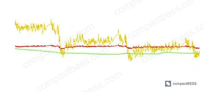
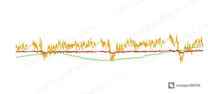
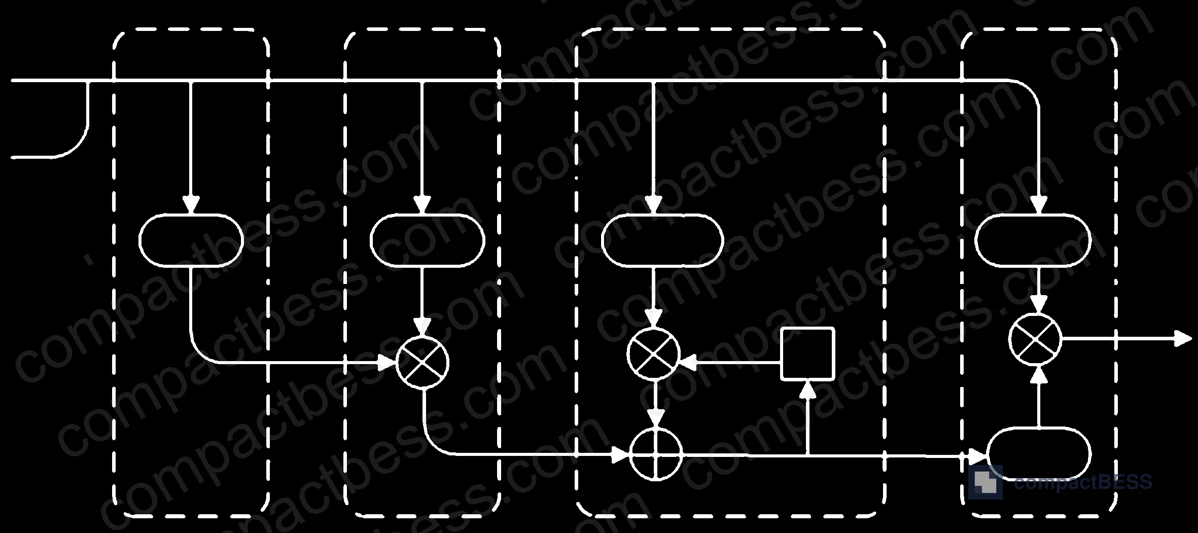
The LSTM-EKF hybrid addresses both weaknesses simultaneously. EKF runs first, generating not just an SOC estimate but also the Kalman gain matrix and state variable update error — which become the training dataset for the LSTM layer. The LSTM then learns to correct EKF residuals rather than estimating SOC from scratch. LSTM network training used 300 iterations, with RMSE stabilizing below 0.02 at iteration 50 and holding there — meaning the network converges quickly and doesn’t require massive training runs. Two LSTM hidden layers with 256 and 128 nodes respectively, plus Dropout layers at probabilities of 0.3 and 0.2, prevented overfitting without excessive computational cost.
The result: SOC error reduced to below 1% across the full test window. In energy storage containers where the aggregate SOC determines grid dispatch commands, that’s the difference between a cell imbalance that’s manageable and one that triggers premature balancing cycles or BMS fault shutdowns.
Thevenin Model Parameter Identification and What Buyers Should Verify #
Honestly, most buyers over-specify neural network capabilities while completely ignoring whether the supplier’s BMS actually has a validated equivalent circuit model underneath. The hybrid algorithm is only as good as the Thevenin model feeding it.
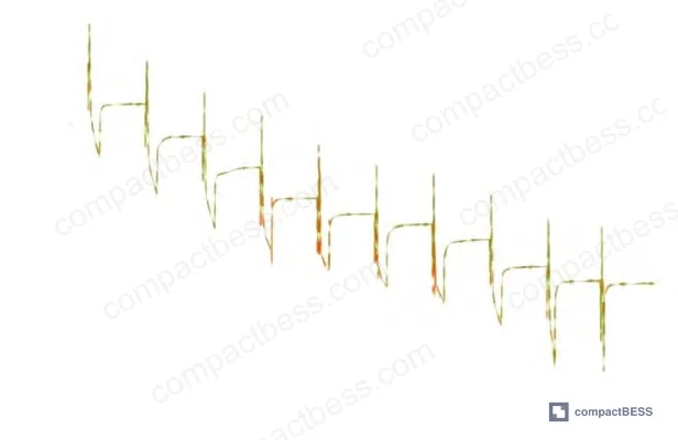
The parameter identification work here was done via HPPC testing — a structured pulse discharge protocol that isolates ohmic resistance (R1) from polarization resistance (R2) and capacitance (C2) by analyzing voltage response across distinct discharge phases. The key values identified for the test cell at representative SOC points:
- At SOC = 0.5: R1 = 0.232 Ω, R2 = 0.013 Ω, C2 = 1,592.6 F
- At SOC = 0.1 (near-empty): R1 = 0.228 Ω, R2 = 0.014 Ω, C2 = 3,720.6 F — notably higher capacitance, reflecting increased polarization at low SOC
- At SOC = 0.8: R1 = 0.221 Ω, R2 = 0.018 Ω, C2 = 1,286.3 F
The OCV-SOC relationship was mapped across the full SOC range from 0.1 (UOC = 3.44 V) to 1.0 (UOC = 4.15 V), fitted using MATLAB’s CFtool. The shape of that curve matters: between SOC 0.3 and 0.8, the voltage gradient is relatively flat (3.57 V to 3.92 V), which is exactly the region where open-circuit voltage methods struggle to resolve SOC accurately. This is why buyers should never accept an OCV-only SOC method specification from a BMS supplier for containerized storage — the flat middle region of the discharge curve makes OCV measurements ambiguous over the majority of the usable SOC window.
The polarization “hysteresis effect” — voltage lagging due to R2 — was directly observed in the HPPC discharge curves as two characteristic phases: a zero-state response at discharge start and a zero-input response at discharge end. Suppliers who can explain these phases and show corresponding R2/C2 identification data understand the physics of their own BMS. Those who can’t are reselling someone else’s firmware.
Containerized BESS Architecture and Algorithm Deployment #
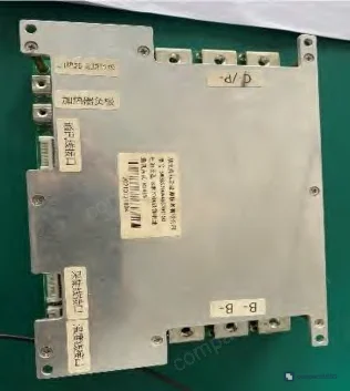
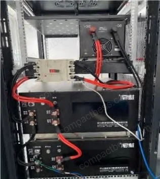
The real-world deployment context in this research deserves attention because it represents the application tier most relevant to grid-scale buyers. The system-level hardware used for algorithm validation was a 5 kW / 10 kWh storage cabinet — the fundamental building block of larger containerized systems. Each cabinet contained two parallel battery boxes, each box built from 8 series-connected cells at 3.2 V nominal per cell. Each battery box had its own dedicated BMS, with an STM32F103 microcontroller as the core processor, two isolated CAN communication channels, and corresponding ADC and I/O ports.
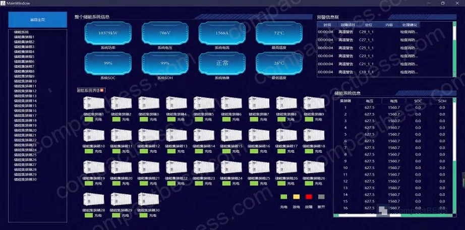
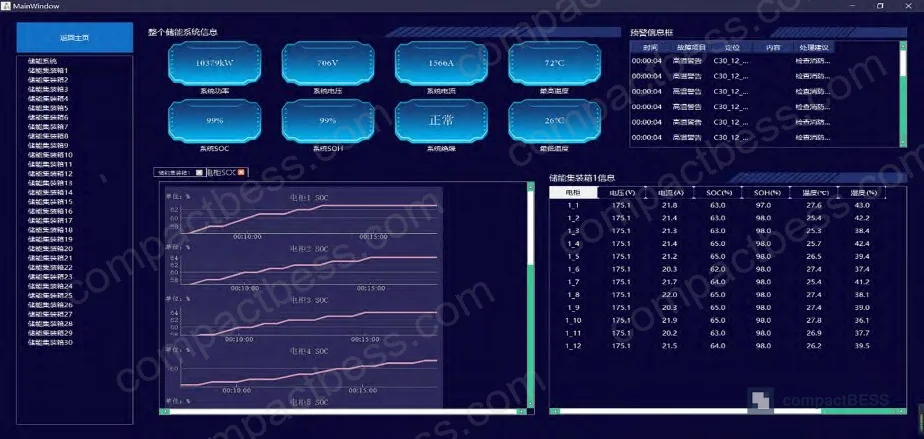
The LSTM-EKF algorithm ran directly on this hardware, collecting voltage and current, computing SOC, and transmitting cell and cabinet-level data to the monitoring platform via CAN bus — consistent with how production containerized BESS systems actually operate. This isn’t a lab-only result. The algorithm was validated on a working hardware platform with a bidirectional PCS managing energy flow.
Most procurement teams don’t realize that the BMS architecture for containerized storage is fundamentally different from EV or portable applications. In containerized BESS, SOC estimation must cascade from individual cell → cabinet → container, with each tier aggregating data upward. An EKF-only BMS might perform adequately at single-cell bench level but accumulate unacceptable error when thousands of cells are aggregated under grid dispatch conditions. The hybrid approach keeps error bounded at the cell level, which prevents error amplification as data propagates up the system hierarchy.
Practical Guidance for Buyers #
If you’re sourcing BMS modules for containerized lithium BESS applications — whether for grid-tied solar storage, industrial UPS, or peak-shaving installations — the SOC algorithm specification is not a checkbox item. It’s a performance-determining parameter that directly affects dispatch accuracy, cell balancing frequency, and cycle life.
Require suppliers to specify: which algorithm, what training dataset, what test conditions, and what maximum SOC error under dynamic load. “Coulomb counting with OCV correction” is not sufficient for containerized storage. “EKF-based estimation” is better but still leaves open-loop risk under high-noise grid conditions. The hybrid approach described here — or a functionally equivalent model-plus-data architecture — should be your baseline for any BMS destined for multi-cabinet containerized BESS.
At CompactBESS, we connect global OEM buyers and energy storage integrators with verified Chinese manufacturers of BMS modules, cell packs, and containerized storage systems — including suppliers with demonstrated hybrid SOC algorithm implementations validated on production hardware. If you’re at the point of supplier shortlisting or technical RFQ preparation, our sourcing team can help you identify manufacturers who can actually answer the questions below.
Need help identifying qualified suppliers for BMS modules with validated SOC estimation? Talk to our sourcing team →
Supplier Qualification Questions #
- What is your maximum SOC estimation error under UDDS-equivalent dynamic load conditions, and can you provide error curves comparing your algorithm output against measured reference SOC values? Threshold: error must be demonstrably below 1% across the full SOC operating window.
- Does your BMS implement a Thevenin or higher-order equivalent circuit model, and can you provide HPPC-derived parameter identification results showing R1, R2, and C2 values at minimum five SOC setpoints between 10% and 90%?
- If your SOC algorithm includes a neural network component, what is the RMSE of the training validation — and at what iteration count does RMSE stabilize? The research benchmark here is RMSE < 0.02 achieved by iteration 50 out of 300.
- How does your EKF or Kalman-based estimator behave when system noise covariance Q and R are set to 1.0 versus 0.5? Can you demonstrate SOC error curves under both noise conditions, showing that error remains bounded rather than diverging?
- What is the validated maximum terminal voltage simulation error between your equivalent circuit model output and measured cell voltage across the full charge/discharge cycle? The reference threshold from validated Thevenin model testing is ≤2.5% relative error.
Sourcing Checklist #
- [ ] BMS specification document states maximum SOC error ≤1% under dynamic (not constant-current) test conditions, with test method explicitly referenced
- [ ] Supplier can provide HPPC test data with offline parameter identification results for R1, R2, and C2 across at least 5 SOC points (e.g., 10%, 30%, 50%, 70%, 90%)
- [ ] OCV-SOC lookup table or fitted curve covers full SOC range from 0.1 to 1.0, with minimum 10 measurement points confirming voltage resolution in the flat region (SOC 0.3–0.7, approx. 3.57–3.82 V for NMC/NCR chemistry)
- [ ] BMS hardware platform confirmed to include isolated CAN communication (≥2 channels) with ADC sampling sufficient for voltage and current measurement at cell level — consistent with IEC 62619 functional safety requirements for battery management
- [ ] Algorithm validation was performed under a recognized dynamic drive cycle (UDDS, WLTP, or equivalent per ISO 12405-4) rather than constant-current discharge only
- [ ] If a neural network component is used, supplier can confirm Dropout regularization or equivalent overfitting prevention, and provide training/validation RMSE convergence data
- [ ] BMS conforms to IEC 62619:2022 safety requirements for stationary lithium battery applications, with test report from accredited third-party lab
- [ ] SOC output is transmitted via CAN or RS485 in real time to higher-level monitoring system, with protocol documentation available for integration review
Key Specifications Table #
| Parameter | Recommended Value | Verification Method |
|---|---|---|
| Maximum SOC estimation error (dynamic load) | <1% across full SOC range | Algorithm simulation under UDDS-equivalent current profile; compare estimated vs. coulometer-reference SOC |
| Thevenin model terminal voltage simulation error | ≤2.5% relative error | Load HPPC-identified R1/R2/C2 parameters into equivalent circuit; compare simulated vs. measured terminal voltage across full discharge |
| LSTM training RMSE at convergence | <0.02 (stabilized by iteration 50 of 300) | Monitor RMSE loss curve during training; confirm plateau before 50 iterations |
| Ohmic internal resistance R1 (at mid-SOC, 0.5) | ~0.232 Ω (cell-level, 18650 format) | HPPC pulse test; calculate from voltage step at discharge start/end using Ohm’s law |
| Polarization capacitance C2 (at SOC = 0.1) | ~3,720 F (elevated vs. mid-SOC) | HPPC zero-input response phase fitting using exponential decay curve in MATLAB CFtool |
| Cell rated capacity (test reference) | 2,250 mAh | IEC 62133 or GB/T 18287 standard capacity test at 0.2C discharge to cutoff voltage |
| SOC initial estimation error (EKF convergence) | Converges from SOC=1.0 initial condition | Set P0=1, monitor state estimate convergence within first 500 s of UDDS input |
Can’t find a supplier meeting these specs? Submit your requirements and we’ll match you within 48 hours.
References #
Data source: Hybrid LSTM-EKF Algorithm for Optimized Cell-Level SOC Estimation in Lithium Battery Energy Storage Container Systems, J. Liu et al., Journal of the Electrochemical Society, 2024
Frequently Asked Questions #
Why does SOC estimation accuracy matter more in containerized BESS than in EV or portable applications?
In a containerized grid storage system, a single installation can contain thousands of cells cascaded across multiple cabinet and container tiers. SOC error at the cell level propagates upward through that hierarchy — a 3% cell-level error can translate into meaningful dispatch inaccuracy at the container level, triggering unnecessary balancing cycles that consume energy and accelerate cell aging. EVs have a single pack with direct monitoring; containerized BESS compounds the problem by scale.
What’s wrong with using open-circuit voltage (OCV) alone for SOC estimation in energy storage applications?
The fundamental problem is the flat discharge curve between SOC 0.3 and 0.7. In the validated OCV-SOC data from this testing, UOC only spans from approximately 3.57 V to 3.82 V across that range — a 250 mV spread over 40% of usable capacity. Sensor noise and measurement uncertainty at that resolution make OCV-based discrimination unreliable. OCV methods also require long rest periods (typically 1+ hour) to reach equilibrium, which is operationally impractical in active grid storage systems.
What does “UDDS conditions” mean and why is it used for battery SOC testing?
UDDS (Urban Dynamometer Driving Schedule) is a standardized current profile originally developed for vehicle emissions testing that includes frequent acceleration and deceleration events — making it a useful proxy for dynamic, non-constant load conditions. For grid storage, the charge/discharge profile from frequency regulation and peak-shaving is similarly irregular. Testing SOC algorithms under UDDS provides a more realistic evaluation of algorithm robustness than constant-current benchmarks, which is why it’s used as the reference input in this evaluation.
Can the LSTM-EKF approach run on low-cost embedded hardware, or does it require high-performance compute?
The hardware deployment in this research used an STM32F103 microcontroller — a 32-bit ARM Cortex-M3 device with no dedicated DSP or neural accelerator. The LSTM network (2 hidden layers, 256 and 128 nodes, with Dropout) ran successfully on this platform alongside real-time CAN communication and data acquisition. The key enabler is that the LSTM is relatively compact and the EKF residuals (not raw cell data) are its primary input, reducing data dimensionality significantly. This means the approach is compatible with mainstream BMS MCU hardware already in production use.
How should I evaluate a BMS supplier’s SOC algorithm claims during supplier qualification?
Ask for three specific outputs: an error curve showing estimated vs. reference SOC under a dynamic test profile (not just a final accuracy number), HPPC parameter identification data confirming they actually characterized the cell they’re using (not just assumed generic values), and RMSE convergence data from training if a neural component is involved. Suppliers who have done this work will have these files. Those who haven’t will offer a datasheet number with no supporting evidence. See the SOC estimation methods documentation and BMS communication protocols guides for deeper evaluation frameworks.
Published by compactbess.com Technical Team | Request a sourcing quote


