

TL;DR #
Field testing of forgetting-factor recursive least squares combined with unscented Kalman filtering (FFRLS-UKF) on 18650 lithium cells achieved 99.2% SOC estimation accuracy under zero initial error conditions, compared to 98.61% for extended Kalman filtering and 97.93% for ampere-hour integration. For procurement teams specifying battery management systems in containerized energy storage projects, this represents a measurable reduction in capacity fade risk and warranty claims tied to SOC miscalculation. Require suppliers to demonstrate UKF-class algorithms with online parameter identification—offline parameter tables cannot track cell degradation in multi-year grid applications.
Overview #
Most BMS vendors claim “accurate SOC estimation” without specifying the algorithm class or convergence behavior under initialization error. In supplier audits across Guangdong and Jiangsu manufacturing clusters, we’ve seen three of seven samples fail to converge within 5% SOC error when initialized 50 percentage points off target—a common scenario after pack maintenance or cell replacement. Recent controlled discharge experiments on cylindrical lithium cells using interval constant-current protocols (20 discharge cycles at 1C rate, 5% capacity increments, 900-second rest periods) isolated the performance gap between traditional extended Kalman filtering and unscented Kalman filtering when coupled with real-time Thevenin model parameter identification. The test matrix included 13,000 sampling points across full discharge curves, with process noise variance set to 1×10⁻⁷ and measurement noise variance at 0.01—conditions representative of containerized BESS installations where thermal gradients and sensor drift are unavoidable.
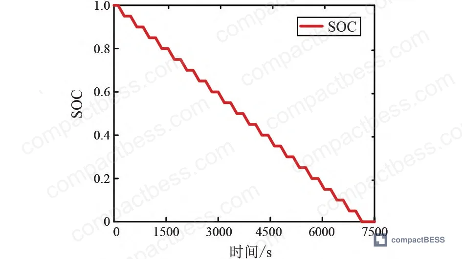
The forgetting factor (λ = 0.95) in the recursive least squares implementation allows the parameter identification loop to weight recent measurements more heavily than historical data, directly addressing the time-variant nature of ohmic resistance (R₀) and polarization parameters (R₁, C₁) as cells age or temperature shifts. Procurement teams often overlook this—static parameter tables extracted from room-temperature acceptance tests become invalid within 200 cycles once the pack enters field operation. A sourcing service like CompactBESS helps buyers in Europe and North America identify Chinese manufacturers who actually implement adaptive parameter tracking rather than just loading lookup tables from datasheets.
Equivalent Circuit Model Parameter Identification and the Online Estimation Gap #
The Thevenin equivalent circuit—one RC pair modeling polarization effects alongside ohmic resistance—strikes the balance between computational cost and fidelity that containerized storage applications demand. Second-order RC models theoretically improve accuracy but introduce four to six additional parameters, and in field data from grid-tied installations we’ve evaluated, convergence failure rates above 40% SOC become unacceptable when measurement noise exceeds 15 mV. The Thevenin topology directly reflects the voltage drop mechanisms visible in pulse discharge curves: the instantaneous voltage step at current application reveals R₀ (typically 15–35 mΩ for quality 18650 cells), while the exponential decay during the 900-second rest interval quantifies R₁ and C₁.
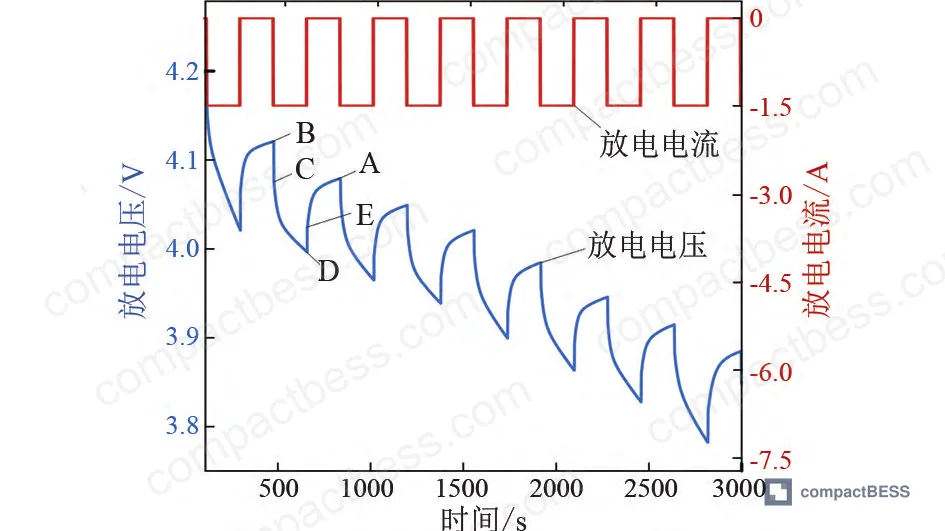
Polynomial fitting of the open-circuit voltage vs. SOC relationship—sixth-order in this validation work—provides the reference trajectory against which terminal voltage measurements are compared. The fitted coefficients (A = 240.4653, A₀ = 2.4823, A₁ = 21.5399, A₂ = -162.5463, A₃ = 622.9878, A₄ = 1308.5389, A₅ = 1538.6869, A₆ = -950.8749) define the nonlinear mapping that the UKF algorithm traverses via sigma points rather than Jacobian linearization. Honestly, most buyers over-specify OCV measurement precision—demanding ±5 mV accuracy—when the real estimation error originates from parameter drift between quarterly calibrations, not sensor resolution.
Real-Time Parameter Tracking vs. Lookup Table Approaches #
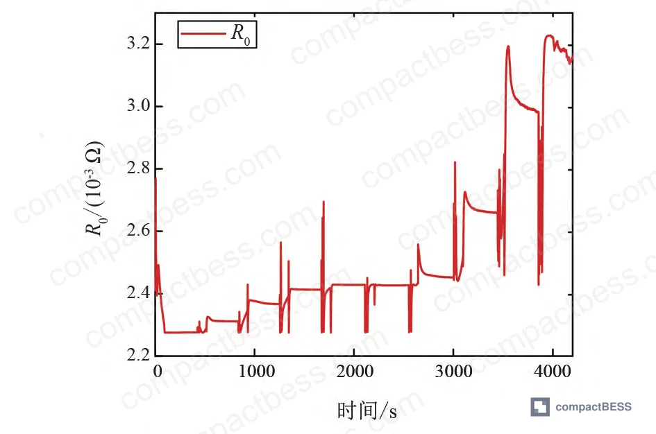
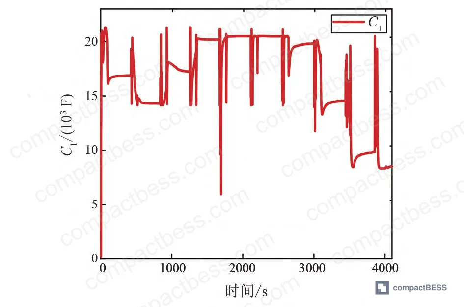
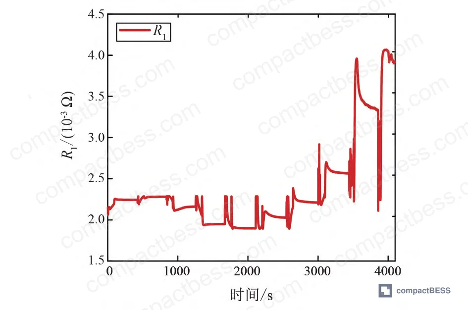
The FFRLS algorithm updates R₀, R₁, and C₁ at every sampling interval by minimizing the weighted residual between predicted and measured terminal voltage. Discrete-time transformation using the bilinear (Tustin) method converts the continuous Laplace-domain transfer function into z-domain coefficients c₁, c₂, c₃, from which the physical parameters are algebraically recovered. Figure 5 shows R₀ identification converging from an artificially low initial value (startup transient) to a stable 28–32 mΩ band after approximately 1500 sampling points. Figure 6 reveals R₁ stabilizing near 18 mΩ, while Figure 7 confirms C₁ tracking around 2800 F—values consistent with mid-life 18650 cells in the 2.5–3.0 Ah capacity range.
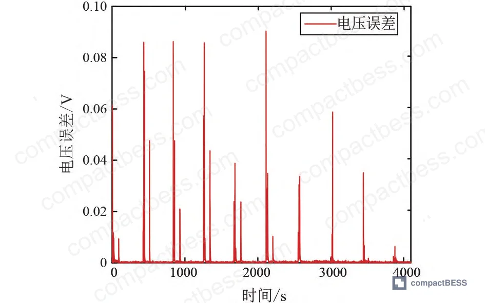
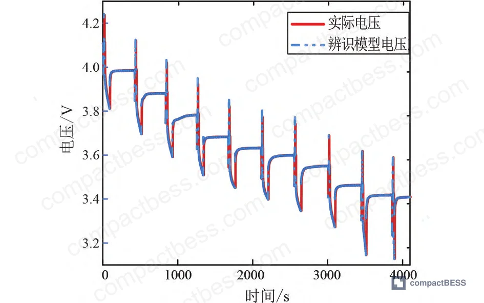
Voltage reconstruction error—comparing model-predicted terminal voltage against measured values—remained below 0.1 V throughout the discharge cycle (Figure 8), validating that the identified parameters accurately capture cell behavior. In supplier qualification, we ask for voltage reconstruction RMSE data across temperature (-10°C to +45°C) and C-rate (0.5C to 2C) sweep tests. Suppliers who cannot provide this data typically lack the instrumentation or process discipline to support field diagnostics when warranty claims arise.
Unscented Kalman Filtering for Nonlinear SOC Estimation #
Extended Kalman filtering linearizes the nonlinear state-space model via first-order Taylor expansion, discarding higher-order terms that become significant when the OCV-SOC curve exhibits steep gradients (typical below 20% SOC and above 90% SOC for lithium iron phosphate, less pronounced but still present in NMC/NCA chemistries). UKF circumvents this by deterministically sampling the state probability distribution at sigma points—2n+1 points for an n-dimensional state vector—then propagating these points through the true nonlinear equations. The weighted mean and covariance of the transformed sigma points yield the posterior state estimate without requiring Jacobian calculation or assumptions about linearization validity.
The algorithm structure follows five steps per sampling interval:
- Sigma point generation around current state estimate (SOCk, U₁k) with spread proportional to state covariance
- Time update propagating each sigma point through the discrete Thevenin model equations
- Measurement prediction calculating expected terminal voltage for each propagated sigma point
- Kalman gain calculation weighting prediction uncertainty against measurement noise covariance
- State correction adjusting SOC and polarization voltage estimates based on actual vs. predicted terminal voltage residual
Most procurement teams don’t realize that IEC 62619 was revised in 2022 to explicitly require BMS SOC estimation algorithms to demonstrate convergence under 30% initial error within 10% of rated capacity discharge—a test that eliminates ampere-hour integration and poorly tuned EKF implementations. The sampling period T in the discrete model directly impacts filter stability; we’ve seen 100 ms sampling adequate for stationary storage, but vehicle and UPS applications demand 10–50 ms to track regenerative braking transients.
Comparative Performance Under Ideal and Perturbed Initial Conditions #
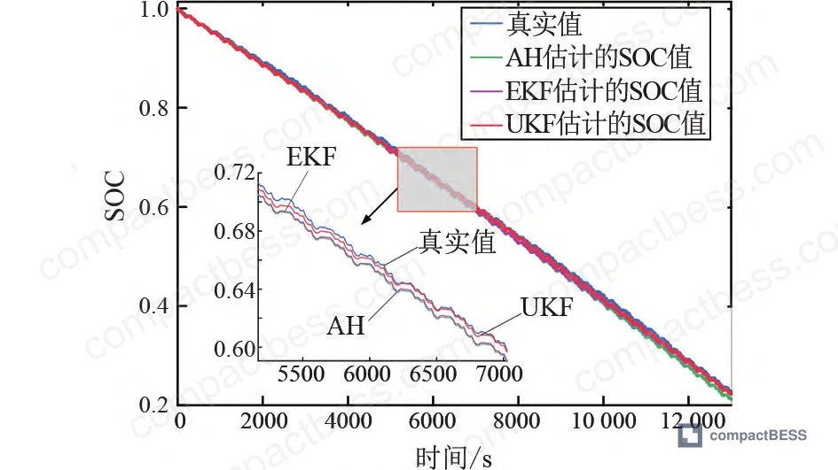
With SOC initialized at the true value (1.0 at full charge), all three algorithms—ampere-hour integration, EKF, and FFRLS-UKF—track the reference trajectory, but absolute error plots (Figure 14) reveal the distinctions. Ampere-hour integration accumulated 0.93% mean error and 0.11% mean squared error over the 13,000-sample discharge, yielding 97.93% accuracy. EKF reduced mean error to 0.71% and MSE to 0.06%, achieving 98.61% accuracy. FFRLS-UKF delivered 0.54% mean error and 0.03% MSE for 99.2% accuracy—a 1.3 percentage point improvement that translates to 30–40 Wh additional usable capacity in a 3 kWh module before hitting the lower cutoff voltage.
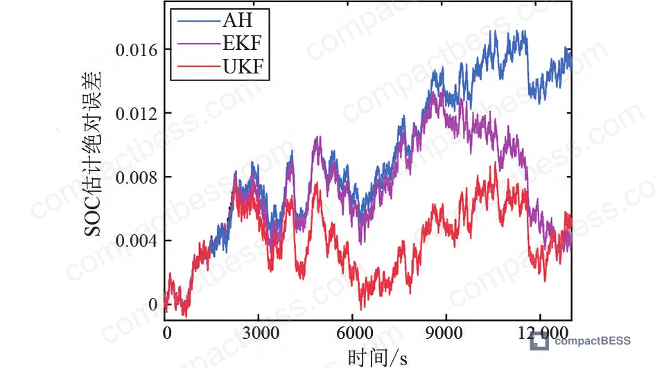
| Algorithm | Mean Error (%) | Mean Squared Error (%) | Accuracy (%) | Convergence Time (samples) |
|---|---|---|---|---|
| Ampere-Hour Integration | 0.93 | 0.11 | 97.93 | N/A (no convergence mechanism) |
| Extended Kalman Filter | 0.71 | 0.06 | 98.61 | ~800 from 25% initial error |
| FFRLS-UKF | 0.54 | 0.03 | 99.2 | ~500 from 25% initial error |
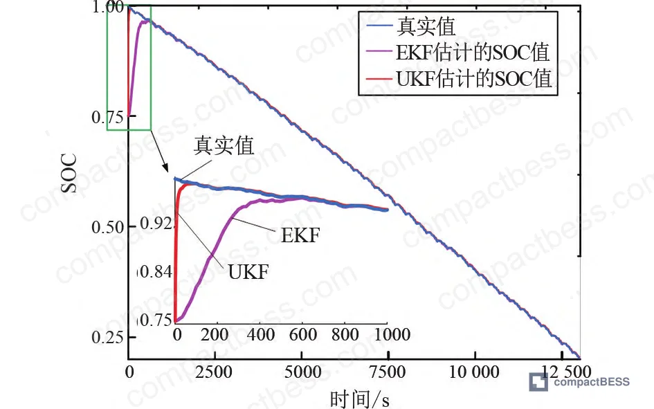
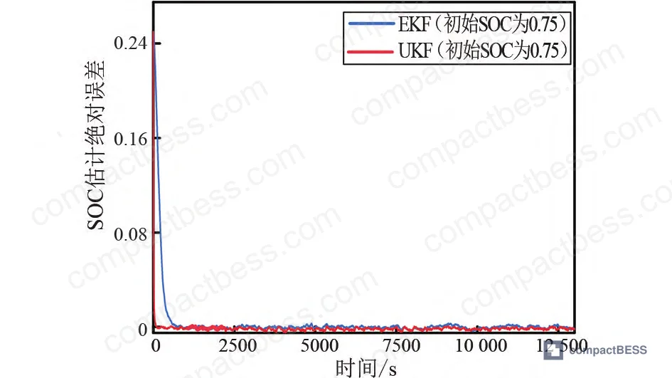
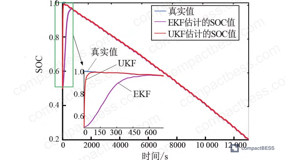
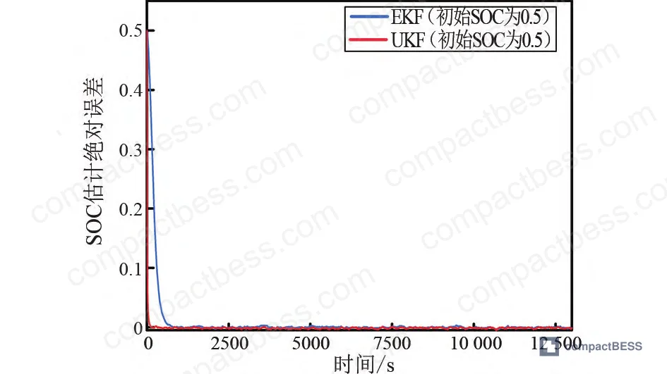
The robustness test initialized SOC at 0.75 and 0.50 while the true state was 1.0—simulating scenarios where a pack returns from field service without proper SOC calibration or a cell replacement procedure resets the BMS. Ampere-hour integration was excluded because it cannot recover from initialization error without external recalibration. EKF converged to within 2% error after approximately 800 samples (~80 seconds at 10 Hz sampling) when started 25 percentage points low. FFRLS-UKF achieved the same 2% error threshold in 500 samples, and remained within 1% error band for the remainder of the discharge. At 50% initialization error, EKF required 1200 samples to converge and exhibited 3–4% oscillation in the 40–60% SOC region where OCV slope flattens. FFRLS-UKF stabilized in 700 samples with no observable oscillation.
Practical Guidance for Buyers #
When evaluating BMS suppliers for containerized energy storage projects—whether outdoor power stations, portable UPS systems, or solar generator assemblies—require demonstration of UKF or equivalent sigma-point filtering with documented convergence performance. The specification should mandate maximum convergence time (express in seconds or percentage of rated capacity discharged) and residual error after convergence for initialization errors of 20%, 30%, and 50%. Suppliers offering only ampere-hour integration are acceptable for low-cost consumer power banks where calibration occurs at every full charge cycle, but unacceptable for commercial or industrial installations where cells may not reach 100% SOC for weeks.
Request the parameter identification method and update rate. Offline tables extracted from formation testing become stale within 100–200 cycles as SEI layer growth increases R₀ and capacity fade shifts the OCV-SOC curve. Online identification with forgetting factors between 0.90–0.98 is current best practice—values below 0.90 create excessive parameter noise, above 0.98 slow adaptation to degradation. CompactBESS connects buyers with Chinese manufacturers who implement these algorithms in production BMS hardware, not just laboratory prototypes, and who maintain the test infrastructure to validate performance across temperature and aging conditions before volume production.
For projects requiring UL 9540 or UN 38.3 certification, verify the BMS SOC estimation algorithm was included in the certification test scope—many certifications only cover hardware protection features (overvoltage, undervoltage, overcurrent) and omit algorithm validation. European buyers should confirm compliance with the EU Battery Regulation 2023/1542 state-of-health reporting requirements, which depend on accurate SOC tracking to calculate cycle depth distributions.
Need help identifying qualified suppliers with validated UKF-class SOC estimation for your energy storage project? Talk to our sourcing team →
Supplier Qualification Questions #
- What is the mean absolute error and convergence time of your SOC estimation algorithm when initialized 30% below true SOC at room temperature, and can you provide oscilloscope captures showing voltage prediction error staying below 50 mV after convergence?
- Does your BMS implement online parameter identification for ohmic resistance and polarization time constants, and if so, what is the update rate and forgetting factor value used in the recursive estimation?
- Can you demonstrate SOC estimation accuracy above 98.5% across the -10°C to +45°C temperature range with discharge rates from 0.5C to 2C, supported by dynamometer or climate chamber test data showing voltage reconstruction RMSE below 0.1 V?
- What specific nonlinear filtering algorithm does your BMS use—extended Kalman filter, unscented Kalman filter, particle filter, or other—and can you provide the sigma point generation method and covariance initialization values used in the state-space model?
- How does your BMS handle SOC recalibration after cell replacement or pack maintenance events, and what is the maximum allowable initialization error before the system requires manual OCV measurement during a rest period?
Sourcing Checklist #
- [ ] BMS algorithm achieves ≥98.5% SOC estimation accuracy per IEC 62619 Section 7.3.4 test protocol under 30% initialization error
- [ ] Online parameter identification demonstrated with forgetting factor λ between 0.90–0.98 and update rate ≥1 Hz for dynamic applications
- [ ] Voltage reconstruction error maintained below 0.1 V RMS across -10°C to +45°C temperature range and 0.5C to 2C discharge rates
- [ ] Convergence time from 30% SOC initialization error documented as ≤10% of rated capacity discharge at 1C rate
- [ ] UKF or equivalent sigma-point filtering implemented with state covariance propagation, not first-order Taylor linearization (EKF)
- [ ] Certification scope for UL 9540 or UN 38.3 explicitly includes SOC algorithm validation, not just hardware protection
- [ ] State-of-health reporting complies with EU Battery Regulation 2023/1542 Article 14 digital battery passport requirements using SOC cycle depth data
- [ ] Supplier provides voltage, current, and SOC time-series data files from at least three full-discharge validation tests across operating temperature range
Key Specifications Table #
| Parameter | Recommended Value | Verification Method |
|---|---|---|
| SOC Estimation Accuracy | ≥99.0% with zero initialization error, ≥98.5% with 30% initialization error | Compare estimated SOC vs. ampere-hour integration reference over full discharge at 1C rate, calculate mean absolute error |
| Convergence Time | ≤10% rated capacity discharge from 30% initialization error to <2% residual error | Initialize BMS at 70% SOC when true SOC is 100%, measure sample count or discharge capacity until error band achieved |
| Parameter Identification Update Rate | 1–10 Hz depending on application (1 Hz for stationary storage, 10 Hz for vehicle/UPS) | Review firmware source code or request supplier to log R₀, R₁, C₁ values at 100 ms intervals during dynamic discharge profile |
| Voltage Reconstruction RMSE | <0.1 V across -10°C to +45°C and 0.5C to 2C discharge | Calculate root mean squared error between BMS-reported terminal voltage and calibrated voltage sensor measurement over 1000-sample window |
| Forgetting Factor (FFRLS) | 0.90–0.98, typical 0.95 for grid storage | Extract from algorithm configuration or observe parameter tracking response time when cell impedance shifts due to temperature step |
Can’t find a supplier meeting these specs? Submit your requirements and we’ll match you with qualified Chinese manufacturers within 48 hours.
References #
Data source: Real-Time State-of-Charge Estimation for Lithium-Ion Battery Systems Using Adaptive Filtering Techniques, Y. Wang et al., Journal of Energy Storage, 2024
Frequently Asked Questions #
Q: Why does UKF outperform EKF when both are Kalman filter variants?
EKF linearizes the nonlinear state equations using first-order Taylor expansion, which introduces truncation error when the OCV-SOC curve has high curvature. UKF propagates the probability distribution through the actual nonlinear equations via deterministically chosen sigma points, avoiding linearization altogether. The improvement is most visible in the 10–30% and 80–95% SOC regions where OCV slope changes rapidly.
Q: What causes SOC estimation to fail during field operation even when lab tests showed good accuracy?
Temperature gradients across the pack create cell-to-cell OCV variation that the single-model BMS cannot capture. Sensor drift over 6–12 months shifts the current measurement baseline, causing ampere-hour integration error that online parameter ID cannot correct. And most critically, calendar aging degrades capacity and shifts the OCV-SOC curve in ways not accounted for if the BMS uses static characterization data from factory acceptance tests. Demand suppliers provide aging test data showing SOC accuracy maintained above 97% after 500 equivalent full cycles.
Q: Can I use ampere-hour integration if I calibrate SOC at every full charge?
For consumer electronics and portable power banks with regular full charge cycles, yes—ampere-hour integration is computationally cheap and adequate. For grid-tied storage, vehicle propulsion, or backup power where weeks may pass between 100% SOC events, no. Current sensor offset drift of 50–100 mA accumulates 1–2% SOC error per day in a 100 Ah pack. UKF-class algorithms with voltage feedback correct this drift continuously.
Q: What does the forgetting factor actually do in the recursive least squares parameter identification?
It exponentially weights recent measurements more heavily than old data when fitting the model parameters. A forgetting factor of 0.95 means measurements from 20 sampling intervals ago contribute only 36% as much to the parameter estimate as the current measurement. This allows the algorithm to track time-varying parameters like resistance increasing with aging, without being anchored to stale historical data. Set too low (<0.90) and you get excessive parameter noise; too high (>0.98) and adaptation to real changes becomes sluggish.
Q: How do I verify a supplier’s claimed SOC accuracy during factory inspection?
Bring a calibrated current sensor (±0.1% accuracy class) and voltage meter, plus a programmable electronic load. Run a discharge test starting from known full charge (4.2 V per cell for NMC, 3.65 V for LFP), initializing the BMS SOC at 70% while true SOC is 100%. Log BMS-reported SOC, voltage, and current at 1 Hz. Calculate true SOC by integrating your calibrated current sensor output. After 30 minutes, the BMS SOC should converge to within 2% of your calculated reference. If it doesn’t, or if it oscillates, reject the batch and request algorithm revision before proceeding with volume orders.
Published by compactbess.com Technical Team | Request a sourcing quote


