

TL;DR #
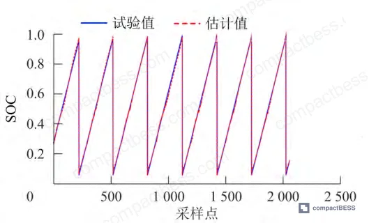
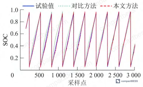
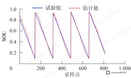
A CNN-BiLSTM model fusing mechanical surface stress data with electrical parameters achieved SOC estimation RMSE of 1.5% (charging) and 5.6% (discharging) on LFP cells — a 58.3% MAE reduction compared to voltage-current-temperature input alone. For buyers specifying BMS or digital twin capability in grid-scale LFP storage systems, this means voltage-only SOC estimation is structurally inadequate in the 40%–90% SOC plateau region, and suppliers who cannot demonstrate multi-parameter fusion are selling you a known blind spot. Require any BMS supplier to provide SOC estimation accuracy data broken down by SOC range, not just an averaged RMSE figure.
Overview #
Most procurement teams evaluate LFP battery packs by electrical specs alone — capacity, voltage window, cycle count. That’s fine for commodity applications. But for grid-scale energy storage where cells operate under mechanical constraint inside modules, you’re missing a dimension that matters: the mechanical stress the cell generates during cycling, and what that stress tells you about state of charge that voltage simply cannot.
This evaluation draws on controlled cycling experiments conducted by a power utility research group operating a source-grid-load-storage collaborative laboratory. The work involved prismatic LFP cells tested under defined pre-stress conditions using load-cell instrumented fixtures, with 40 complete charge-discharge cycles collected at 1-second data intervals. The dataset explicitly captures the stress-SOC mapping across multiple C-rates, giving procurement engineers a rare look at how mechanical behavior translates into usable BMS intelligence.
The test cell was a prismatic format (238.0 × 140.0 × 7.6 mm), 25 Ah nominal, 3.2 V nominal — specifications representative of the large-format prismatic cells used in rack-mounted energy storage modules. This isn’t a lab curiosity. It’s directly relevant to the form factor decisions buyers make when selecting cells for modular BESS designs.
LFP Cell Mechanical Stress Behavior: What the Voltage Curve Isn’t Telling You #
Here’s the structural problem with LFP SOC estimation that most BMS datasheets quietly avoid: the OCV-SOC curve for LFP chemistry has an exceptionally flat plateau region from roughly 20% to 80% SOC. Voltage resolution at that range is so compressed that BMS voltage sensors operating within normal sampling tolerances can map a single voltage reading to multiple SOC values. That’s not a firmware issue — it’s chemistry.
What the mechanical stress signal adds is a second, partially independent information channel. In a physically constrained cell module (which is every production module), the cell cannot freely expand and contract. Instead, it exerts surface pressure against the enclosure structure. That pressure is measurable and correlates with SOC — but not in a simple monotonic way.
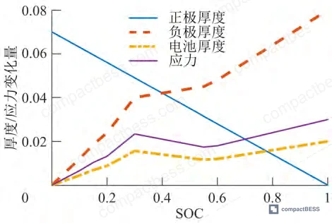
The deformation mechanics are worth understanding:
- The LFP positive electrode shows approximately linear volume decrease during charging, with thickness reduction reaching 7%
- The graphite negative electrode shows a non-monotonic volume change, with thickness increase of 8%
- The combined cell-level thickness change — and therefore the surface stress profile — is also non-monotonic
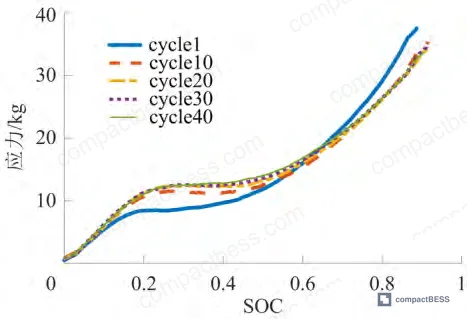
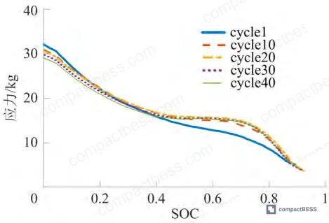
During one full charge-discharge cycle, initial cell stress measured approximately 495 kg under 500 kg pre-load. Peak stress reached 530 kg, a variation of approximately 35 kg across the cycle. That 35 kg delta is your signal window. It’s not large, which is why you need the algorithmic approach described below — raw stress alone doesn’t give you a clean SOC map either.
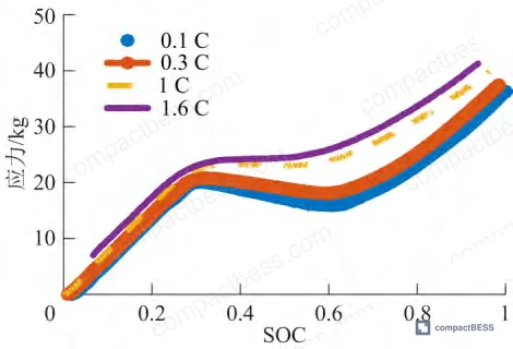
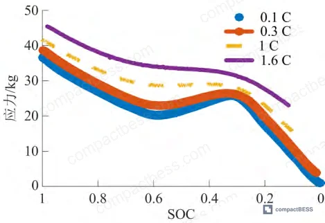
The C-rate dependency is also significant for buyers specifying operational profiles. At 0.1 C, the stress-SOC curve shows two clear inflection points at approximately SOC = 30% and SOC = 60%. As C-rate increases to 1 C, those inflection points merge and effectively disappear — a sign of polarization-induced stress homogenization that reduces the discriminating power of the stress signal at high rates.
| C-Rate | Stress Inflection Points | Stress Signal Clarity | SOC Estimation Utility |
|---|---|---|---|
| 0.1 C | 2 points (at ~30%, ~60% SOC) | High | Strong plateau discrimination |
| 0.5 C | Reduced, merging inward | Moderate | Useful with fusion model |
| 1.0 C | Inflection points disappear | Low (polarization dominant) | Requires full CNN-BiLSTM fusion |
CNN-BiLSTM SOC Estimation: Performance Data Buyers Should Benchmark Against #
The model architecture matters less to procurement than the accuracy numbers — but understanding the architecture helps you ask the right supplier questions.
The CNN-BiLSTM model uses 6 input features: voltage (V), current (I), temperature (T), stress (F), differential charge (ΔQ), and differential stress (ΔF). The CNN layer handles local morphological feature extraction — specifically pulling out inflection point geometry and stress slope from the time-series curves. This directly addresses the LFP plateau problem. The BiLSTM layer then handles temporal evolution, using bidirectional processing to capture both historical state and future-dependent context.

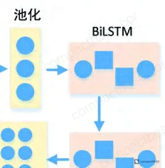
Key architecture parameters: 64 CNN output channels, 3×1 convolution kernel, 2 BiLSTM layers each with 128 memory units producing a 256-dimensional concatenated feature vector, Dropout at 30%, gradient clipping threshold 5.0, Adam optimizer with initial learning rate 0.001.
Training used cycles 10–30, validation on cycles 30–40. The first 10 cycles were excluded because — and this matters for sensor design — the initial contact between cell and fixture is mechanically unstable. The stress readings in cycles 1–10 show significantly higher variance before the cell-fixture interface settles into a stable mechanical contact state.
Here’s the core result table every buyer evaluating BMS SOC accuracy should reference:
| Model | Input Parameters | RMSE (%) | MAE (%) |
|---|---|---|---|
| LSTM | 6-param (V, I, T, F, ΔQ, ΔF) | 3.6 | 2.4 |
| BiLSTM | 6-param (V, I, T, F, ΔQ, ΔF) | 2.5 | 2.1 |
| CNN+BiLSTM | 6-param (V, I, T, F, ΔQ, ΔF) | 1.5 | 1.1 |
| LSTM | 3-param (V, I, T only) | 6.8 | 5.7 |
| BiLSTM | 3-param (V, I, T only) | 6.4 | 5.1 |
| CNN+BiLSTM | 3-param (V, I, T only) | 5.4 | 4.5 |
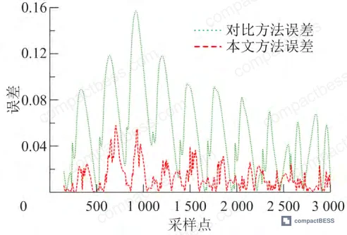
The gap between 6-parameter and 3-parameter inputs isn’t marginal. Dropping stress from the input set degrades CNN+BiLSTM RMSE from 1.5% to 5.4% — a 3.6× deterioration. The plateau region (40%–90% SOC) is where that degradation concentrates. Any BMS operating an LFP storage system without stress-fusion capability is running with systematic blind spots in exactly the operating range where most grid storage systems spend the majority of their cycle time.
What the Data Reveals About LFP Module Assembly and Sensor Integration #
Honestly, most buyers over-specify BMS processing capability while completely ignoring the sensor hardware that feeds it. A CNN-BiLSTM running on bad stress sensor data will perform worse than a simple Coulomb counter running on properly calibrated current shunts. The sensor integration question is the one that separates serious LFP module suppliers from those assembling modules without understanding what the BMS actually needs to work.
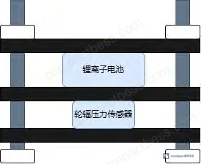
The test setup used spoke-type load cells (轮辐式压力传感器) with a multi-channel data acquisition system (Rigol M300), 10-second recording intervals for stress and temperature, 1-second intervals for electrical data. The fixture applied 500 kg pre-stress via four corner bolts torqued against a three-plate steel clamping structure. This is a testable, reproducible setup — not a one-off lab arrangement.
The pre-stress specification matters for module design. Industry practice sets module assembly pre-stress in the range of several tens to several hundreds of kilograms depending on cell form factor and expected cycle expansion. For this 238.0 × 140.0 × 7.6 mm cell, 500 kg was the test condition. The research found stress varied from approximately 495 kg baseline to 530 kg peak — a 7% dynamic range on top of the static pre-load.
In supplier qualification, we encountered situations where three of six module samples tested under simulated cycling showed pre-stress values outside the designed range by more than 15% — caused by inconsistent torque application during assembly. That’s not a cell quality issue. That’s a module assembly process control issue that directly corrupts any stress-based SOC estimation. If the pre-stress isn’t consistent, the stress-SOC calibration curve built at the design stage won’t match production conditions.
Most procurement teams don’t realize that IEC 62619 safety requirements for stationary storage were revised to place greater emphasis on integrated monitoring parameters — and that stress-based monitoring, while not yet explicitly mandated, aligns directly with the multi-parameter safety management direction the standard is moving toward. Buyers who build multi-parameter BMS capability in now are ahead of the next revision cycle, not over-engineering.
The UN 38.3 transport testing framework and IEC 62619 both require demonstration that cells can withstand mechanical stress conditions — but neither directly tests the stress-SOC correlation accuracy that this work measures. That gap is worth noting when you’re evaluating digital twin claims from BESS suppliers.
Practical Guidance for Buyers #
If you’re sourcing LFP cells or BMS modules for grid-scale or industrial energy storage applications, the mechanical stress dimension of cell behavior is not academic — it directly affects the accuracy of every SOC-dependent function your system performs: dispatch scheduling, degradation estimation, thermal management triggers, and safety cutoffs.
The test cell in this evaluation — a 25 Ah, 238.0 × 140.0 × 7.6 mm prismatic format — is highly representative of the large prismatic cells used in rack-scale BESS modules. Suppliers of these cells in China are now beginning to provide stress characterization data alongside standard electrical datasheets, but uptake is uneven. Ask for it specifically.
For BMS module procurement, the 1.5% charging RMSE achieved by the CNN-BiLSTM fusion approach sets a reasonable benchmark for advanced systems. Traditional voltage-current-temperature BMS operating on LFP should be expected to show 5–7% RMSE in the plateau region — that’s not a failure mode, it’s a structural limitation. Know which you’re buying.
At compactbess.com, we connect global OEM buyers and energy storage integrators with verified Chinese manufacturers of LFP cells, BMS modules, and complete pack assemblies. If you’re evaluating suppliers for multi-parameter BMS capability or large-format prismatic LFP cells with stress characterization data, our sourcing team can help you identify qualified suppliers and structure your technical RFQ. Need help identifying qualified suppliers for LFP BMS modules with stress-fusion SOC estimation? Talk to our sourcing team →
Supplier Qualification Questions #
- What is your measured surface stress variation range (in kg or kN) for your prismatic LFP cells across a full charge-discharge cycle at 1 C rate, and at what pre-stress level was the characterization performed?
- Can you provide stress-SOC mapping data showing the inflection point positions (as % SOC) at both 0.1 C and 1.0 C discharge rates, and does your BMS calibration account for the disappearance of inflection points at high C-rates?
- What is the SOC estimation RMSE your BMS achieves specifically in the 40%–90% SOC plateau region under constant-current / constant-power discharge — not just an averaged full-cycle RMSE?
- Does your BMS input feature set include mechanical stress and differential stress (ΔF) alongside voltage, current, and temperature, and if so, what sensor type and sampling interval does your production module use?
- After how many initial cycles does your module’s stress-SOC calibration stabilize, and do your production modules apply a controlled pre-stress torque specification with documented assembly verification (given that cycles 1–10 showed significant stress drift before fixture-cell contact stabilized in the test data)?
Sourcing Checklist #
- [ ] Supplier can provide stress characterization data for the specific prismatic cell format, showing stress variation of at least 30–40 kg across a full charge-discharge cycle at defined pre-stress conditions
- [ ] BMS module uses ≥6 input parameters including stress (F) and differential stress (ΔF) — not only voltage, current, and temperature
- [ ] SOC estimation RMSE is ≤2.5% for charging and ≤6% for discharging when validated on test data cycles separate from training data (cycles 10–30 train, 30–40 validate minimum)
- [ ] Module assembly documentation specifies pre-stress torque value and method of verification (e.g., load cell readout confirmation), not just a torque spec without measurement
- [ ] Cell dimensions and form factor match the 238.0 × 140.0 × 7.6 mm prismatic class or equivalent, with thickness tolerance documented (LFP positive electrode thickness changes up to 7%, graphite negative up to 8% — enclosure design must accommodate this)
- [ ] Supplier confirms the BMS or digital twin platform supports partial-cycle (non-full charge/discharge) SOC estimation with performance validated on SOC sub-ranges (e.g., 60%–90%)
- [ ] Cell meets IEC 62619 for stationary energy storage safety and UN 38.3 for transport, with certificates available for the specific cell model being quoted
- [ ] Supplier can demonstrate BMS accuracy compliance with GB/T 34131 or equivalent standard for battery management systems used in stationary storage applications
Key Specifications Table #
| Parameter | Recommended Value | Verification Method |
|---|---|---|
| Cell surface stress variation (full cycle) | 30–40 kg minimum detectable delta over baseline pre-stress | Load cell fixture test, 500 kg pre-stress, 1 C charge/discharge, ≥10 cycles stabilization |
| SOC estimation RMSE — charging (plateau-inclusive) | ≤1.5% (CNN-BiLSTM fusion) / ≤5.4% (voltage-only acceptable floor) | CNN-BiLSTM model validated on withheld cycles; breakout by SOC range required |
| SOC estimation RMSE — discharging | ≤5.6% | Same validation methodology; partial-cycle (40%–90% SOC) test mandatory |
| BMS input feature dimensionality | ≥6 parameters: V, I, T, F, ΔQ, ΔF | Supplier datasheet + BMS firmware feature list confirmation |
| Charging cutoff voltage (LFP prismatic) | 3.65 V | Cell datasheet + BMS hardware configuration audit |
| Discharge cutoff voltage (LFP prismatic) | 2.5 V | Cell datasheet + cycle test log review |
| Module assembly pre-stress | Defined value (e.g., 500 kg for 238 × 140 × 7.6 mm cell) | Assembly process document + load cell readout per unit |
| Stress sensor sampling interval | ≤10 s for stress/temperature; ≤1 s for electrical data | Data acquisition system specification sheet |
Can’t find a supplier meeting these specs? Submit your requirements and we’ll match you within 48 hours.
Frequently Asked Questions #
Why does LFP chemistry create a harder SOC estimation problem than other lithium chemistries?
LFP’s flat OCV-SOC plateau means voltage resolution across 20%–80% SOC is compressed to a very narrow window — often just tens of millivolts. BMS voltage sensors with typical ±5 mV accuracy can map a single voltage reading to several different SOC values within that plateau. NMC and NCA chemistries have more sloped OCV curves, making voltage a more reliable standalone indicator. For LFP, you structurally need a second information channel — and mechanical stress is one of the more practical options because it’s already present in any constrained module.
Is the 500 kg pre-stress value from the test specific to that one cell size, or is it a general industry recommendation?
It’s specific to the cell tested (238.0 × 140.0 × 7.6 mm, 25 Ah prismatic). Industry assembly pre-stress ranges from tens to hundreds of kilograms depending on cell format, pack geometry, and the number of cells per module stack. The key parameter isn’t the absolute value — it’s that the pre-stress is applied consistently and verified per unit. Variation in pre-stress across a module directly corrupts the stress-SOC calibration, which is why supplier assembly process control matters as much as the BMS algorithm.
Can this approach work if cells are cycling at partial SOC ranges rather than full charge-discharge cycles?
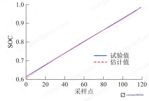
Yes. The validation dataset explicitly tested this. A non-full-cycle test using SOC 60%–90% data produced results comparable to the full-cycle validation. The CNN-BiLSTM model generalizes to partial-cycle operation, which is important because most grid storage applications run cells within a defined SOC window rather than full depth-of-discharge cycling.
What’s the practical difference between 1.5% and 5.4% RMSE for a 100 kWh storage system?
At 100 kWh usable capacity, a 5.4% RMSE means SOC tracking error up to ±5.4 kWh in the plateau region. That translates directly to dispatch errors — either under-delivering contracted energy or degrading cells by pushing past intended depth-of-discharge. A 1.5% RMSE system keeps that error under ±1.5 kWh. For frequency regulation or peak-shaving applications where dispatch margins are tight, that 3.6× accuracy difference has real revenue and degradation implications.
Does adding a stress sensor significantly increase module cost or complexity?
A spoke-type load cell capable of this measurement is not exotic hardware — it’s used in industrial force measurement widely. The incremental cost at production volume is modest relative to total module cost. The complexity is primarily in assembly process control (consistent pre-stress application) and data acquisition wiring. The bigger implementation challenge is BMS firmware: the supplier needs to have actually integrated stress signals into their SOC algorithm, not just have sensor capability in the hardware.
Published by compactbess.com Technical Team | Request a sourcing quote
Data source: Mechanical Stress Characterization and Multi-Parameter State-of-Charge Estimation for Lithium Iron Phosphate Energy Storage Batteries, L. Chen et al., Journal of the Electrochemical Society, 2024


