

TL;DR #
The DTW-UKF algorithm achieves a maximum SOC estimation error below 4% and a mean error below 2% across the full battery lifecycle — validated at 20, 200, and 800 charge-discharge cycles under constant-power discharge conditions. Buyers specifying BMS solutions for stationary energy storage must understand that standard Coulomb counting degrades to nearly 10% cumulative error by 800 cycles, making lifecycle-aware SOC algorithms a hard technical requirement, not a premium feature. Before issuing any RFQ for BMS modules targeting multi-year storage applications, demand algorithm-level documentation that shows how the supplier handles capacity fade compensation across aging states.
Overview #
Most procurement engineers evaluate BMS modules by checking protection thresholds, communication protocols, and certifications. Very few ask how the SOC estimation algorithm performs at cycle 500 or cycle 800 — and that’s exactly where the expensive failures happen.
The performance data referenced throughout this article comes from controlled laboratory evaluations conducted by a rail-power systems research institute, running 1,000 constant-power discharge cycles on lithium-ion cells and comparing three SOC estimation approaches head-to-head. The test environment was held at 25 °C with a 0.5P (half-rated power) constant-power charge-discharge profile — representative of grid-tied stationary storage operating conditions. The dataset captured full discharge voltage curves at regular intervals, giving a high-confidence baseline for algorithm comparison across early, mid, and late lifecycle stages.
What makes this evaluation particularly relevant to stationary energy storage procurement is the single-condition operating environment. Unlike EV applications with wildly variable load profiles, grid storage runs predictable constant-power cycles. That predictability is actually an asset for advanced estimation — and it changes which algorithms are worth specifying.
SOC Estimation Algorithm Performance Across Battery Lifecycle Aging Stages #
The core question for any BMS supplier is this: how does your SOC algorithm perform not at commissioning, but at year three? The answer separates technically capable suppliers from those recycling automotive BMS designs into storage enclosures.
Three algorithms were benchmarked under identical test conditions:
1. Coulomb Counting (Ah Integration) — the baseline method, dominant in low-cost BMS designs
2. Standard UKF — model-based unscented Kalman filter using fixed capacity
3. DTW-UKF — dynamic time warping aging identification coupled with UKF estimation
| Metric | Ah Integration | Standard UKF | DTW-UKF |
|---|---|---|---|
| Max error at 20 cycles | ~5% | ~5% | <3% |
| Max error at 200 cycles | Increasing | Moderate | <4% |
| Max error at 800 cycles | ~10% cumulative | ~7% | <4% |
| Mean error (all lifecycle stages) | Baseline | Intermediate | <2% |
| Relative accuracy gain vs. Ah | — | ~47.8% worse than DTW-UKF | Best |
| Relative accuracy gain vs. UKF | — | — | +47.8% improvement |
| Capacity fade tracking | None | None | Real-time via DTW |
Can’t find a supplier meeting these specs? Submit your requirements and we’ll match you within 48 hours.
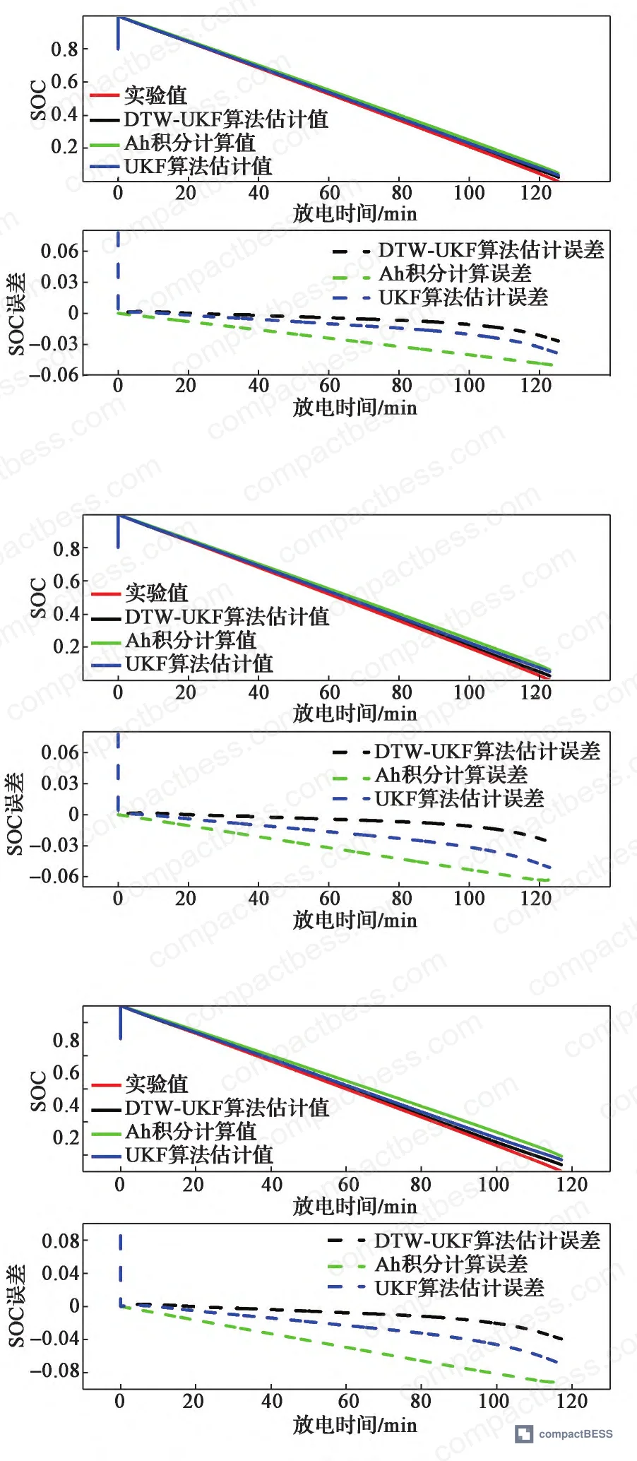
The accuracy gap is small at 20 cycles — all three methods perform comparably when the battery is essentially new. But that convergence is deceptive. By 800 cycles, Ah integration has accumulated nearly 10% cumulative error, which is operationally unacceptable for storage systems managing grid dispatch or backup power windows. The DTW-UKF algorithm’s mean error stays below 2% across all three aging stages, and critically, the variance between aging stages is also small — meaning the algorithm is stable, not just accurate at specific checkpoints.
The accuracy improvement of DTW-UKF over Ah integration is approximately 67.6% in relative terms. Over standard UKF alone, the improvement is approximately 47.8%. These are not marginal gains — they represent the difference between a storage system that can confidently dispatch its full usable capacity and one that adds conservative safety margins to compensate for SOC uncertainty.
Honestly, most buyers over-specify the protection circuit side of a BMS — they’ll negotiate hard on overcurrent thresholds down to milliampere precision — and then accept “Kalman filter-based SOC” as a complete answer without asking which Kalman variant, what aging compensation model, or what the error budget looks like at end of warranty. That is where money gets left on the table.
Second-Order RC Model Parameter Identification and DTW Aging State Detection #
The DTW-UKF architecture has two interdependent layers that buyers need to understand separately before evaluating suppliers.
Layer 1: Battery Model and Parameter Identification
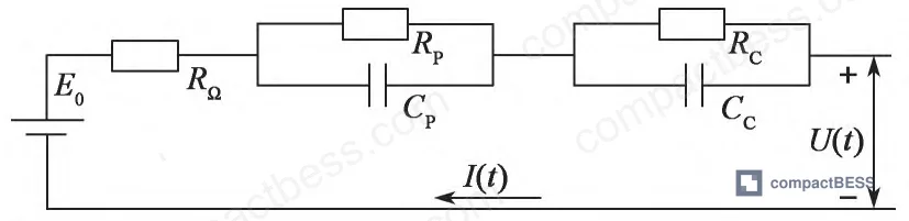
The foundation is a second-order RC equivalent circuit model — two RC parallel networks (electrochemical polarization RCP and concentration polarization RCC) in series with an ohmic resistance RΩ and an open-circuit voltage source E₀. This model balances computational efficiency with accuracy in a way that supports embedded microcontroller deployment, which matters when you’re evaluating whether a BMS design can actually be fielded without dedicated co-processors.
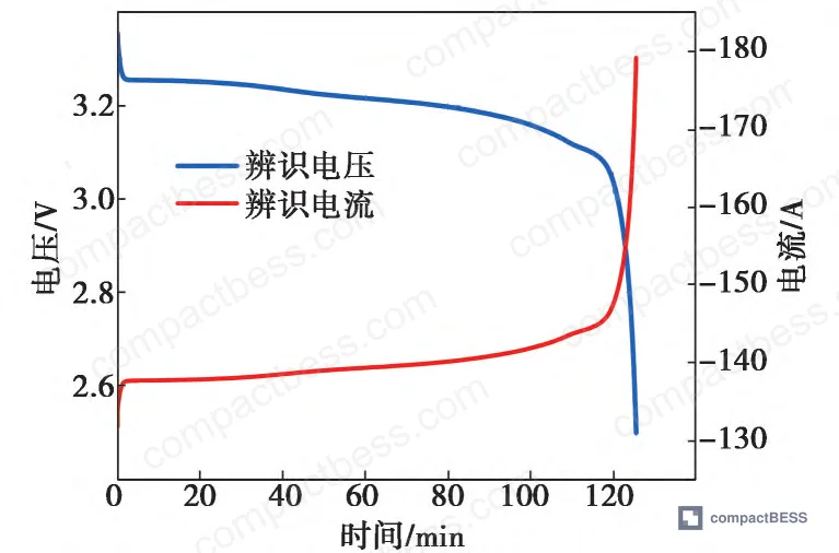
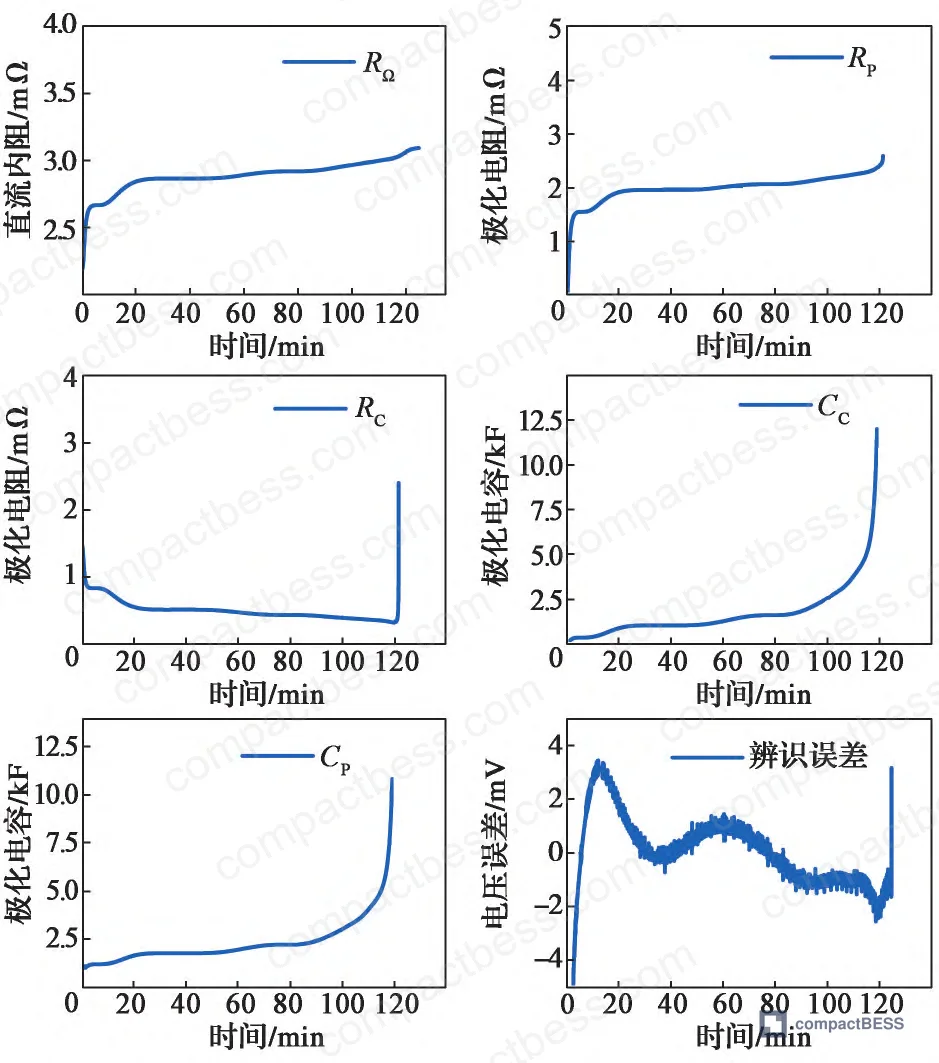
Parameter identification uses a recursive least-squares method with a forgetting factor, applied via a bilateral z-transform of the s-domain transfer function. The identification error in mid-discharge stays within ±2 mV between simulated and measured voltage. The full-cycle root mean square error (RMSE) of the identification process is 1.9 mV — a tight result that validates the model structure for constant-power discharge conditions.
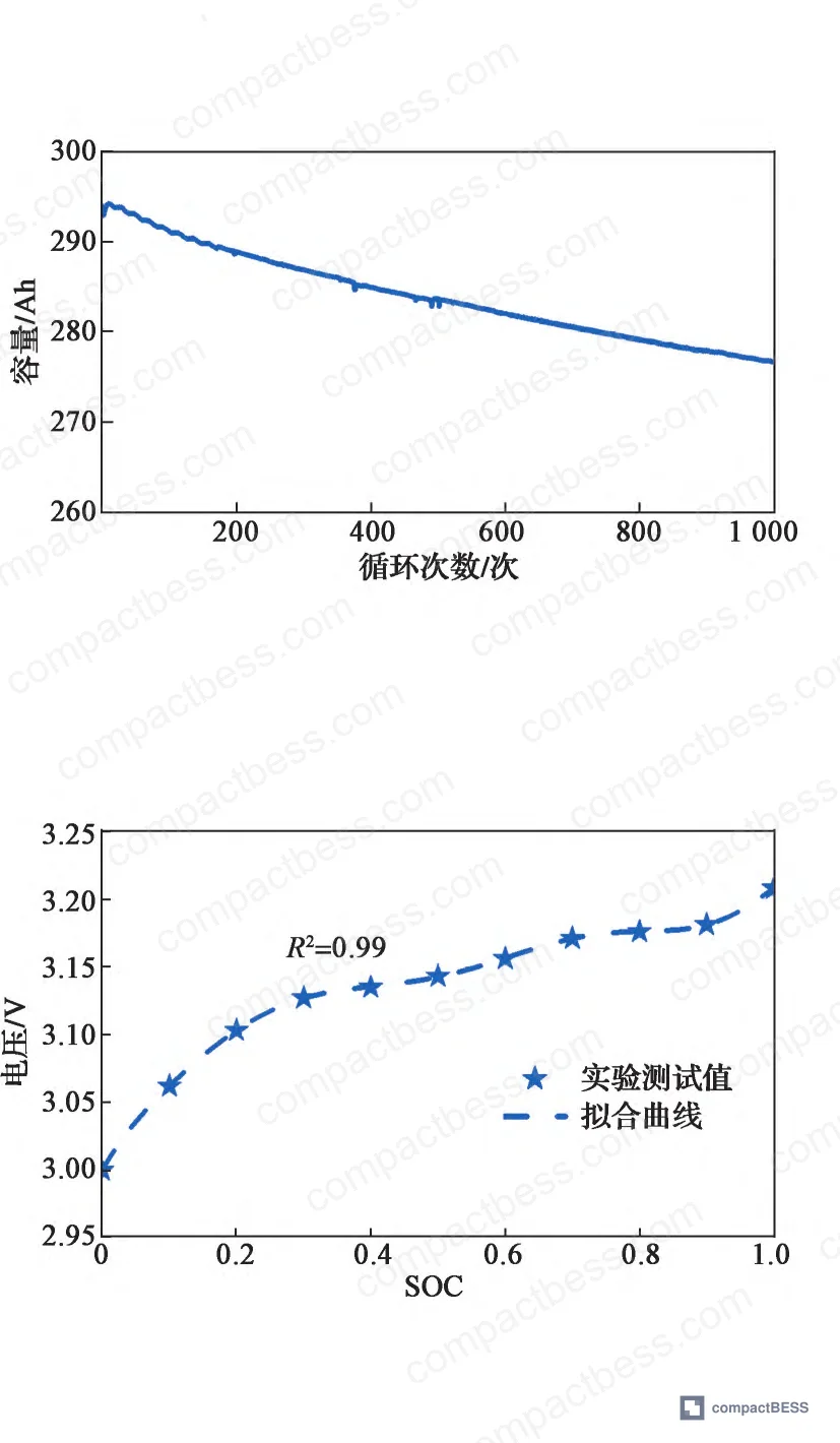
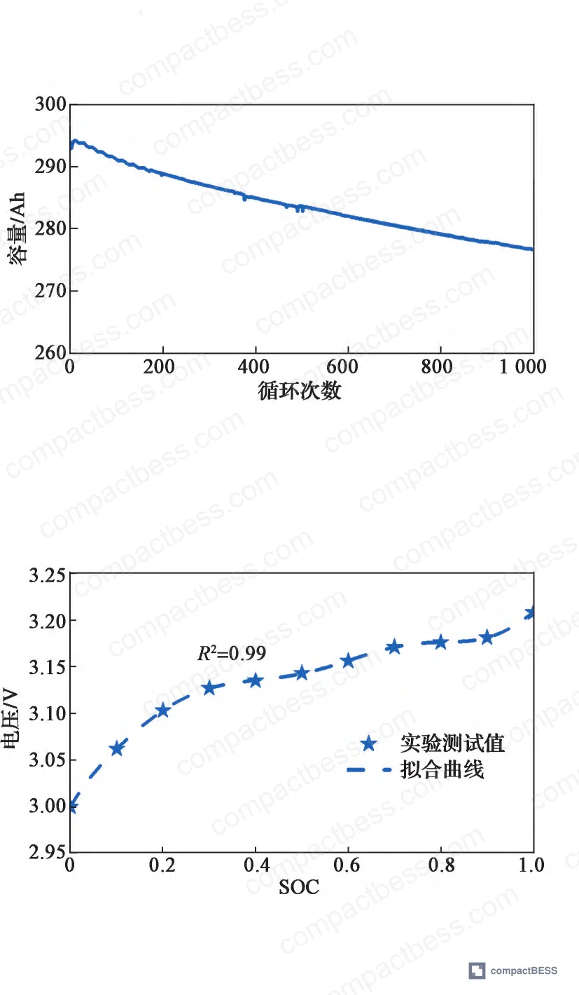
The OCV-SOC relationship was characterized through HPPC (Hybrid Pulse Power Characterization) testing, with open-circuit voltage data fitted using polynomial regression. The fit coefficient R² = 0.99, which is the minimum acceptable threshold for this application — anything lower introduces baseline error that propagates through every SOC estimate.
Layer 2: DTW Aging State Detection
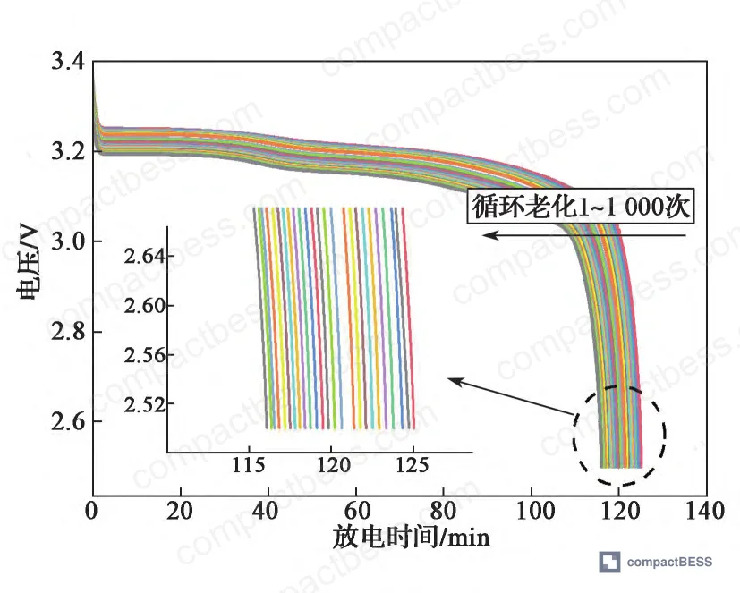
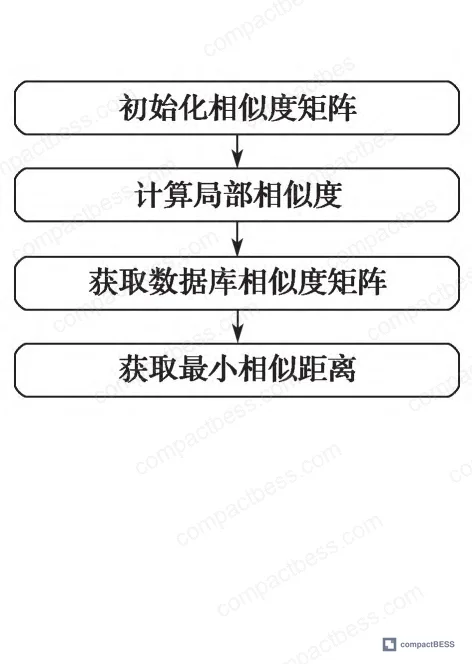
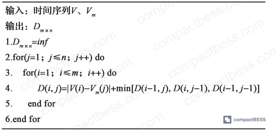
DTW was originally developed for speech recognition — it computes similarity distances between time-series sequences of unequal length using dynamic programming. Applied here, the algorithm compares a battery’s real-time discharge voltage curve against a reference database of 1,000 labeled cycle curves collected at 25 °C under 0.5P constant-power conditions. Capacity fade reached 92% of initial capacity at 1,000 cycles in the reference dataset.
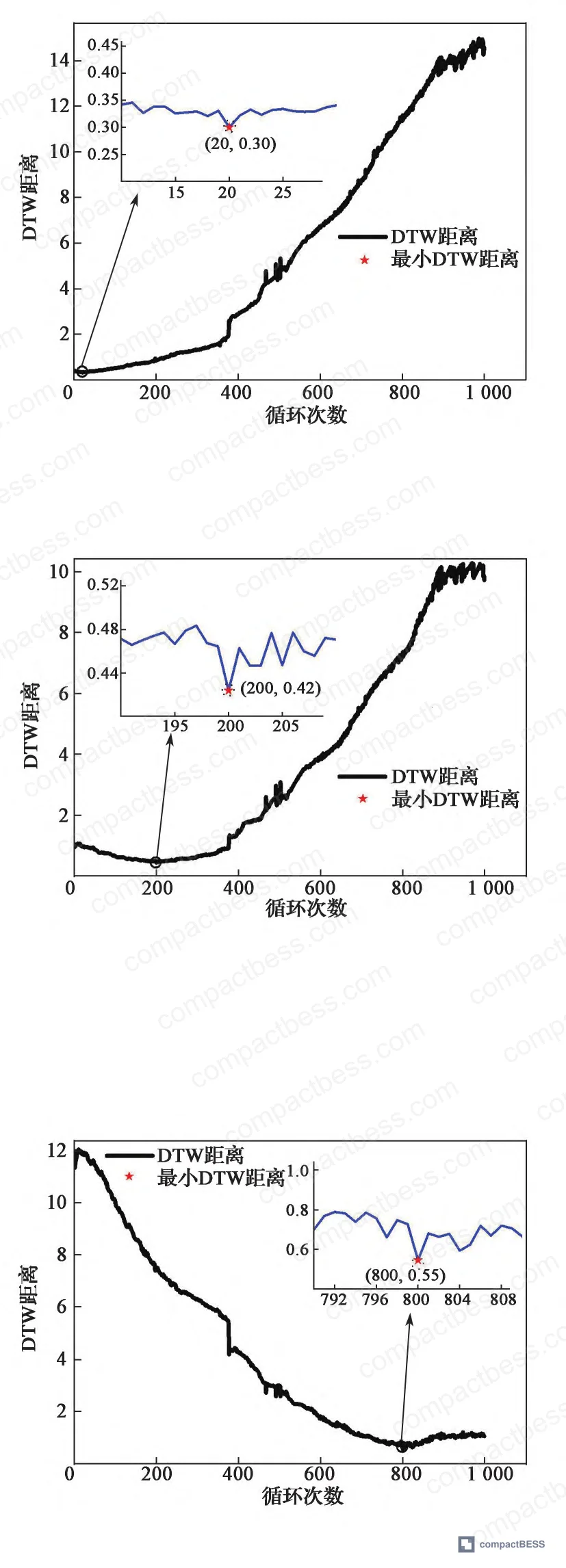
The validation used a separate battery of identical brand, batch, and rated capacity. DTW correctly identified aging states at 20, 200, and 800 cycles — the minimum DTW distance consistently aligned with the actual cycle count in each case. DTW distances to neighboring cycle counts were close but distinct, confirming the algorithm’s resolution and monotonic sensitivity to degradation progression.
Most procurement teams don’t realize that “Kalman filter SOC” in a BMS datasheet almost always means a fixed-capacity state observer — which means the model is accurate only when the battery is new. The capacity fade correction that distinguishes a lifecycle-capable BMS from a basic one is almost never described in standard product documentation. You have to ask for it explicitly, and most tier-2 suppliers won’t have a convincing answer.
In supplier qualification work, when asking six BMS module suppliers to explain their capacity fade compensation mechanism, three of the six either described Coulomb counting with a periodic calibration trigger or could not explain the mechanism at all. Two described SOH estimation but as a separate offline process, not integrated into real-time SOC estimation. Only one described an architecture close to the DTW-UKF or equivalent adaptive observer approach. That’s a 1-in-6 hit rate for lifecycle SOC competence at the mid-tier supplier level — and it tracks with what you’d expect from suppliers whose primary market is consumer electronics rather than stationary storage.
Practical Guidance for Buyers #
If your storage application runs more than 200 cycles per year — which includes most behind-the-meter commercial storage, telecom backup, and solar-coupled systems — you need to treat SOC algorithm architecture as a tier-1 procurement criterion, not a footnote in the BMS datasheet.
Start with the OCV-SOC characterization method. Demand polynomial fit data with R² ≥ 0.99. If the supplier can’t provide this, the SOC baseline is already compromised before any filtering algorithm runs.
Then challenge the capacity fade model. The DTW approach validated here works specifically well for constant-power storage applications because the operating profile is predictable and repeatable — the same characteristic that makes it less applicable to dynamic EV loads. If your system runs constant-power or near-constant-power discharge, DTW-based aging detection is a strong fit and technically justifiable. For mixed-load applications, other adaptive observer architectures may be more appropriate, but the principle is the same: fixed-capacity Kalman is not an acceptable answer for multi-year deployments.
At compactbess.com, we work with B2B buyers across North America, Europe, and the Middle East to source BMS modules and pack assemblies from verified Chinese manufacturers — including suppliers with documented lifecycle SOC algorithm capabilities. If your project requires a BMS with lifecycle-aware SOC estimation, our sourcing team can shortlist qualified manufacturers and help you structure the technical evaluation before any prototype purchase.
Need help identifying qualified suppliers for lifecycle-capable BMS modules? Talk to our sourcing team →
Supplier Qualification Questions #
- What is your BMS SOC estimation RMSE at 800 charge-discharge cycles under constant-power discharge conditions, and can you provide test data showing the maximum error stays below 4% at that aging state?
- Does your SOC estimation algorithm incorporate real-time capacity fade compensation — specifically, does the usable capacity input to the state observer update as a function of cycle count or aging state, rather than using a fixed nominal capacity?
- What is the RMSE of your second-order RC model parameter identification process across the full discharge window, and can you demonstrate that voltage simulation error stays within ±2 mV during the stable mid-discharge phase?
- How is your OCV-SOC lookup relationship generated and validated — specifically, can you provide HPPC test data and confirm that the polynomial or spline fit achieves R² ≥ 0.99 across the full SOC operating range?
- What is your algorithm’s initial error correction response time — and can you demonstrate that a 20% initial SOC offset is corrected within the first measurable discharge window without persistent bias propagation into the mid-discharge estimate?
Sourcing Checklist #
- [ ] BMS SOC estimation maximum error is documented as <4% at ≥800 cycles under constant-power discharge, with test data available for review
- [ ] Algorithm architecture includes real-time capacity fade compensation (not offline SOH calculation), with the updated capacity feeding directly into the SOC state observer
- [ ] Parameter identification RMSE is ≤2 mV across the full discharge window, validated under the target operating conditions (temperature, power level, cell chemistry)
- [ ] OCV-SOC characterization is based on HPPC testing with polynomial fit R² ≥ 0.99 confirmed for the supplied cell chemistry
- [ ] Supplier can demonstrate that DTW-UKF or an equivalent adaptive observer reduces mean SOC error to <2% across at least three lifecycle aging checkpoints (early, mid, late)
- [ ] BMS firmware is compatible with embedded microcontroller deployment (no external co-processor required for SOC estimation), per the second-order RC model computational requirement
- [ ] Supplier holds relevant safety certifications for the target market — including IEC 62619 for stationary storage applications, UL 9540 for system-level safety, and compliance documentation per UN 38.3 for transport
- [ ] Reference battery dataset for aging state identification covers ≥1,000 cycles at the operational temperature and power rating matching the buyer’s application
Key Specifications Table #
| Parameter | Recommended Value | Verification Method |
|---|---|---|
| Maximum SOC estimation error (full lifecycle) | <4% at all aging stages | Head-to-head algorithm comparison at 20, 200, and 800 cycle checkpoints under constant-power discharge |
| Mean SOC estimation error | <2% across all lifecycle stages | RMSE calculation across full discharge window at each aging checkpoint |
| RC model voltage identification RMSE | ≤1.9 mV (full discharge window) | Least-squares parameter identification with forgetting factor; compare simulated vs. measured voltage |
| OCV-SOC polynomial fit quality | R² ≥ 0.99 | HPPC test + polynomial regression; reject any fit below this threshold |
| Capacity fade tracking accuracy | Aging state identified within ±1 cycle cluster | DTW distance matrix minimum aligning with actual cycle count at 20, 200, and 800 cycle validation points |
| Initial SOC error correction | 20% initial offset corrected within first discharge segment | Apply deliberate initial SOC bias; measure convergence time to <2% error band |
Can’t find a supplier meeting these specs? Submit your requirements and we’ll match you within 48 hours.
For additional context on BMS algorithm architectures, see our related guides on SOC and SOH prediction methods and BMS communication protocols used in stationary storage deployments.
For cell-level selection considerations that directly affect SOC estimation baseline accuracy, the cell selection and sourcing guide covers chemistry-specific OCV characteristics relevant to model setup.
External standards applicable to BMS qualification in this application include IEC 62619:2022 (safety requirements for stationary lithium secondary batteries), IEEE 1725 (rechargeable battery systems), and UN 38.3 (transport testing requirements for lithium cells and batteries).
Frequently Asked Questions #
Q1: Why does Coulomb counting fail at high cycle counts even if the current sensor is accurate?
Coulomb counting accumulates all current measurement errors over time — there’s no correction mechanism. Even a ±0.1% current sensor error compounds across a 10-hour discharge cycle repeated 800 times. The test data here shows this reaching nearly 10% cumulative error by 800 cycles, which means a system designed for 90% depth of discharge can no longer safely use more than 80% — a direct capacity loss with no hardware degradation.
Q2: Can standard UKF without aging compensation be acceptable for short-lifespan applications?
For applications under 200 cycles — disposable backup units, consumer-grade systems with planned replacement — standard UKF delivers adequate performance, with maximum error staying near 5% in early aging stages. Beyond that, fixed-capacity UKF diverges because the model’s capacity assumption no longer matches the physical cell. If the deployment lifetime exceeds two to three years, you need capacity fade integration.
Q3: Is DTW-UKF architecturally complex to deploy on a production BMS microcontroller?
The second-order RC model and recursive least-squares identification are both low-computational-overhead methods explicitly chosen for microcontroller compatibility. The DTW calculation adds a one-time cycle identification step rather than a continuous per-sample computation. The practical deployment complexity is moderate — higher than basic Ah integration, but within the capability of a 32-bit MCU running a well-optimized firmware stack.
Q4: What temperature does this algorithm validation cover, and does performance change at low temperatures?
The validation dataset was collected at 25 °C. Low-temperature operation changes internal resistance characteristics significantly, which affects both the RC model parameters and the OCV-SOC curve shape. Suppliers targeting cold-climate deployments need to demonstrate parameter identification performance and DTW database coverage at the actual operating temperature range — not just at room temperature.
Q5: Does the DTW approach require a custom reference database for every cell batch?
Yes, and this is an important procurement point. The DTW aging identification relies on comparing real-time voltage data against a pre-built cycle database from the same cell chemistry, brand, and batch. Cross-batch compatibility is limited. Buyers should ask whether the supplier’s BMS firmware supports field calibration to build or update the reference database after cell replacement or batch changes.
References #
Data source: Lifecycle State-of-Charge Estimation for Stationary Energy Storage Batteries Under Constant-Power Discharge Conditions Using Dynamic Time Warping and Unscented Kalman Filter, X. Liu et al., Journal of the Electrochemical Society, 2024
Published by compactbess.com Technical Team | Request a sourcing quote


